48 Quadrats 3

As we saw in the previous section, it is not clear whether there exists a single grid resolution, or rule for selecting grid resolutions, that performs well across all parameter regimes.

In this section, we therefore focus on selecting a grid (or set of grids) that provides robust discrimination between the LGCP and CSCP across a range of settings.

To do this, we compare candidate grid sets using a simulation-based pilot study. Rather than constructing a formal hypothesis test at this stage, we use a simple classifier as a convenient way to quantify how well the two models can be separated. In this context, classification accuracy serves as a proxy for statistical power: a grid strategy with high classification accuracy is one where the models are easily distinguishable.

Since the aim is not to develop an optimal classifier, but to determine whether the two processes can be separated using observable quadrat-count behaviour, we use a simple distance between empirical quadrat-count distributions as the statistic of classification.

For a given grid resolution \(m\), define

\[ D_m(X; M) = \sum_k \left| \hat p_m(k;X)-\bar p_{M,m}(k) \right| \]

where \(\hat p_m(k;X)\) is the empirical quadrat-count distribution for the observed pattern, and \(\bar p_{M,m}(k)\) is the mean quadrat-count distribution under model \(M\), estimated via simulation. \(\bar p_{M,m}(k)\) acts as an approximation of the true theoretical distribution of quadrats counts.

Note

Why is \(\bar p_{M,m}(k)\), the mean of the simulated-pattern quadrat count distributions, an approximation of the the true distribution?

[Elaborate]

Note

\(\bar p_{M,m}(k)\) is straight nasty notation. Can definitely do better.

For a set of grid resolutions \(\mathcal M\), we define the overall distance

\[ D(X; M) = \sum_{m \in \mathcal M} D_m(X; M) \]

and classify the pattern as the model with the smaller distance.

Note

In simpler terms, \(D(X; M)\) is the sum of the distances of each empirical distribution to the true distribution. That is, for every grid resolution within the grid-set:

Calculate the distance to each of the true distributions.
Then add them all up (so we will end up with two sums, representing the distances from the CSCP and LGCP truth respectively).
Classify based on whichever distance is smallest.

This classification rule is used only within this pilot study to compare grid strategies. In the next section, we use the same distance-based statistic to construct a more formal Monte Carlo hypothesis test.

48.1 Relative grid sizing

There is one last thing we need to address before conducting the study.

Rather than selecting grid resolutions directly, we index candidate grids by the expected number of points per quadrat,

\[ \eta_m = \frac{\lambda |W|}{m^2} \]

This gives a scale-free way to describe grid coarseness. For example, \(\eta_m = 20\) corresponds to a grid where each quadrat contains 20 points on average, regardless of the size of the observation window.

For a target expected quadrat count \(\eta\), the corresponding square grid resolution is

\[ m(\eta) = \left\lceil \sqrt{\frac{\lambda |W|}{\eta}} \right\rceil \]

Note

Should this be floor instead of ceiling?

Thus, candidate grid strategies are defined in terms of sets of expected counts, such as

\[ \mathcal E = \{5, 10, 20, 40\}, \]

rather than fixed values of \(m\). This makes the resulting rule easier to apply outside the simulation setting, where the observation window and intensity may differ.

Below we show an example, where the candidate grid-sets have expected counts \(\{5 \}\) and \(\{5, 20\}\), and \(\lambda = 2000\).

eta_sets <- list(
  "eta_5" = 5,
  "eta_5_20" = c(5, 20)
)

grid_sets <- make_grid_sets_from_eta(
  W = owin(),
  lambda = 2000,
  eta_sets = eta_sets
)
grid_sets

$eta_5
[1] 20

$eta_5_20
[1] 20 10

We can see, we can see the associated grid resolutions for the above expected quadrat counts.

48.2 Pilot design

For each parameter regime, we generate independent training and test sets from both the CSCP and matched LGCP. The training set is used only to estimate the reference quadrat-count distributions \(\bar p_{M,m}\). The test set is then classified using the distance rule above.

We repeat this over a grid of parameter regimes,

\[ \lambda \in \{\cdots\}, \qquad \phi \in \{\cdots\}, \qquad s_{\text{CSCP}} \in \{\cdots\}. \]

For each candidate grid strategy \(\mathcal E\), we record the classification accuracy within each regime, together with its mean, minimum, and interquartile width across regimes.

Since the goal is robustness rather than best-case performance, candidate strategies are ranked primarily by their worst-case accuracy across regimes. Ties are broken using mean accuracy and then interquartile width.

48.3 Pilot

Candidate grid sets:

eta_sets <- list(
  "eta_2" = 2,
  "eta_5" = 5,
  "eta_10" = 10,
  "eta_20" = 20,
  "eta_40" = 40,
  "eta_80" = 80,

  "eta_2_5_10" = c(2, 5, 10),
  "eta_5_10_20" = c(5, 10, 20),
  "eta_10_20_40" = c(10, 20, 40),
  "eta_20_40_80" = c(20, 40, 80),

  "eta_2_5_10_20" = c(2, 5, 10, 20),
  "eta_5_10_20_40" = c(5, 10, 20, 40),
  "eta_10_20_40_80" = c(10, 20, 40, 80),

  "eta_2_5_10_20_40" = c(2, 5, 10, 20, 40),
  "eta_5_10_20_40_80" = c(5, 10, 20, 40, 80),
  "eta_2_5_10_20_40_80" = c(2, 5, 10, 20, 40, 80)
)

And regimes:

regimes <- tidyr::crossing(
  lambda = c(1000, 5000, 10000),
  phi = c(1, 1.5, 2),
  s_cscp = c(0.1)
)

Running the pilot:

eta_grid_results <- run_eta_grid_pilot(
  W = spatstat.geom::owin(c(0, 1), c(0, 1)),
  regimes = regimes,
  eta_sets = eta_sets,
  n_train = 300,
  n_test = 100,
  seed = 789
)

Summarise by regime:

Top candidate grid strategies ranked by worst-case classification accuracy across all parameter regimes.
Expected counts per quadrat	Worst-case accuracy	Mean accuracy	Median accuracy	IQR	Mean LGCP accuracy	Mean CSCP accuracy
{2, 5, 10, 20, 40}	0.720	0.862	0.895	0.125	0.790	0.933
{2, 5, 10, 20}	0.710	0.857	0.875	0.095	0.822	0.891
{2, 5, 10, 20, 40, 80}	0.690	0.849	0.895	0.155	0.739	0.959
{10, 20, 40}	0.680	0.835	0.860	0.200	0.747	0.923
{5, 10, 20, 40}	0.675	0.855	0.870	0.150	0.789	0.921
{2, 5, 10}	0.655	0.832	0.855	0.080	0.806	0.858
{5, 10, 20}	0.645	0.849	0.865	0.130	0.828	0.871
{5, 10, 20, 40, 80}	0.645	0.840	0.865	0.170	0.722	0.958

Best within each regime:

Best-performing candidate grid strategy within each parameter regime.
lambda	phi	s_CSCP	Best expected counts per quadrat	Induced grid resolutions	Accuracy	LGCP accuracy	CSCP accuracy
1000	1.0	0.1	{2, 5, 10}	{10, 14, 22}	0.800	0.77	0.83
1000	1.5	0.1	{2, 5, 10, 20}	{7, 10, 14, 22}	0.830	0.81	0.85
1000	2.0	0.1	{2, 5, 10, 20, 40}	{5, 7, 10, 14, 22}	0.720	0.61	0.83
5000	1.0	0.1	{10, 20, 40}	{11, 16, 22}	0.955	0.94	0.97
5000	1.5	0.1	{5, 10, 20, 40}	{11, 16, 22, 32}	0.870	0.83	0.91
5000	2.0	0.1	{2}	{50}	0.930	0.87	0.99
10000	1.0	0.1	{20, 40, 80}	{11, 16, 22}	0.995	0.99	1.00
10000	1.5	0.1	{10, 20, 40, 80}	{11, 16, 22, 32}	0.940	0.90	0.98
10000	2.0	0.1	{2, 5, 10}	{32, 45, 71}	0.960	0.93	0.99

Interesting that when \(\phi = 2\) and \(\lambda = 5000\), the best grid set is just \(\{2\}\).

Nice plot of results:

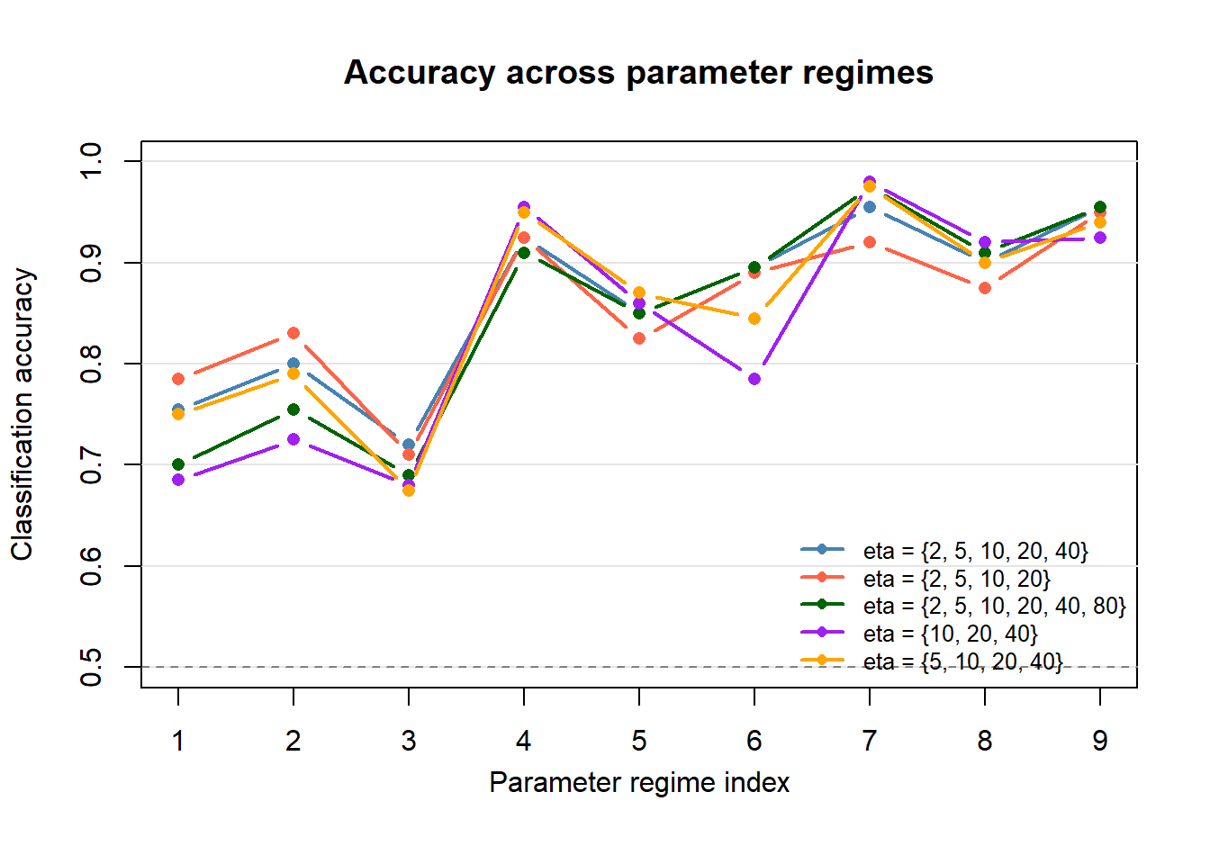
Parameter regimes used in the pilot power study.
Regime index	lambda	phi	s_CSCP
1	1000	1.0	0.1
2	1000	1.5	0.1
3	1000	2.0	0.1
4	5000	1.0	0.1
5	5000	1.5	0.1
6	5000	2.0	0.1
7	10000	1.0	0.1
8	10000	1.5	0.1
9	10000	2.0	0.1