Motivation
In the previous chapter, we introduced the intensity function \(\lambda(u)\) as a fundamental descriptor of first-order structure.
In practice, however, the intensity function is unknown.
Instead, we observe a single realization of a point process:
\[
X = \{x_1, \dots, x_n\}.
\]
From this, we want to estimate \(\lambda(u)\).
This raises a natural question:
How can we estimate a spatially varying function from a single point pattern?
Constant intensity
We begin with the simplest setting.
Suppose the process first-order homogeneous, so that
\[
\lambda(u) = \lambda
\]
Then the expected number of points in the observation window \(W\) is
\[
\mathbb{E}[N(W)] = \lambda |W|.
\]
A natural estimator of \(\lambda\) is therefore
\[
\hat{\lambda} = \frac{N(W)}{|W|}
\]
Interpretation:
- \(N(W)\) is the total number of observed points
- \(|W|\) is the area of the observation window
- so \(\hat{\lambda}\) is simply the observed density of points
This estimator is intuitive, and often works well when the intensity is truly constant.
Suppose the intensity is constant. When would this estimator NOT work well?
However, it completely ignores spatial variation.
If we use the global estimator
\[
\hat{\lambda} = \frac{N(W)}{|W|},
\]
we lose all information about where the points are concentrated within \(W\).
To recover spatial variation, we need a local estimator of \(\lambda(u)\).
A moving window idea
A natural idea is to estimate the intensity near a location \(u\) by counting how many points fall in a small region around \(u\).
Let \(B(u, r)\) denote a ball of radius \(e\) centred at \(u\).
We could define
\[
\hat{\lambda} = \frac{N(B(u, r))}{|B(u, r)|}
\]
This estimates the local density of points near \(u\).
We are approximating
\[
\lambda(u) \approx \frac{\text{number of points near } u}{\text{area of neighbourhood}}
\]
Is this basically quadrat estimation.
Problem with this approach
This estimator depends heavily on the choice of \(r\):
If \(r\) is very small, then the estimate is noisy
If \(r\) is very big, then the estimate is over-smoothed
This trade-off motivates a less sensitive approach.
Kernel intensity estimation
Instead of using a hard cutoff (points inside the ball vs outside), we can use a kernel function to weight nearby points smoothly.
The kernel estimator is
\[
\hat{\lambda} = \sum_{i=1}^n \frac{1}{h^d} K\left( \frac{u - x_i}{h} \right),
\]
where:
- \(K(\cdot)\) is a kernel function (e.g. Gaussian)
- \(h > 0\) is the bandwidth
- \(d\) is the dimension (typically \(d=2\))
- each observed point contributes a “bump” centred at its location
- the total intensity is the sum of these bumps
- nearby points contribute more than distant ones
Common choice: Gaussian kernel
A typical choice is the Gaussian kernel:
\[
K(x) = \frac{1}{2\pi} \exp\left(-\frac{\|x\|^2}{2}\right)
\]
This produces a smooth intensity surface.
The bandwidth parameter
The most important parameter in kernel estimation is the bandwidth \(h\).
It controls the degree of smoothing:
- Small \(h\):
- very detailed estimate
- high variability (noisy)
- Large \(h\):
- smooth estimate
- may obscure important structure
The bandwidth controls the bias–variance trade-off.
Choosing \(h\) too small or too large can lead to misleading conclusions about the underlying process.
In practice, selecting an appropriate bandwidth is a key part of intensity estimation.
Edge effects
A practical issue arises near the boundary of the observation window.
Points near the edge have part of their kernel “falling outside” the window, leading to underestimation of intensity near the boundary.
To correct for this, edge correction methods are used.
Idea:
Adjust the contribution of each point to account for the portion of its kernel that lies outside the observation window.
Most software implementations handle this automatically.
We address this topic as well as bandwidth selection more thoroughly in later chapters.
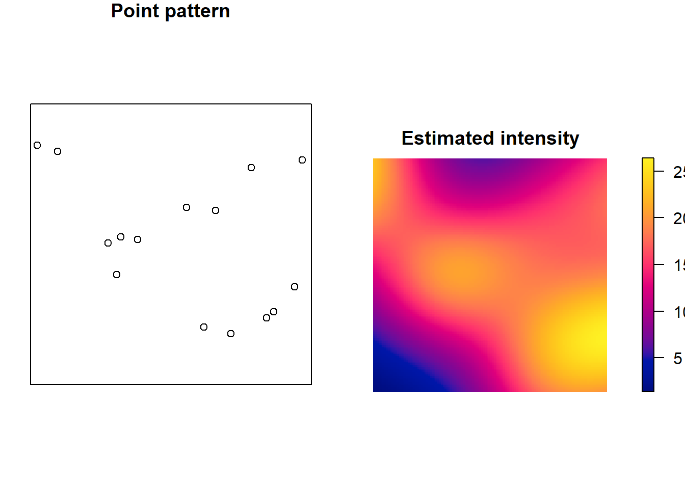
Implementation in R (spatstat)
In spatstat, intensity estimation is performed using the density() function.
Make these plots prettier.
UPDATE – these chunks are being annoying af and won’t load, come back to this.
library(spatstat)

X <- rpoispp(win = owin(), lambda = 20)
lambda_hat <- density(X, sigma = 0.2)

par(mfrow = c(1,2), mar = c(1,1,1,1))

plot(X, main = "Point pattern")
plot(lambda_hat, main = "Estimated intensity", ribargs = list(las = 1), legend = FALSE)
Interpreting intensity estimates
When interpreting an estimated intensity surface:
However care must be taken:
apparent “hotspots” may be due to small bandwidth
smoothing may hide important features
edge effects can distort boundaries if not corrected
Summary
Intensity estimation aims to recover the unknown function \(\lambda(u)\) from an observed point pattern.
- For homogeneous processes:
\[
\hat{\lambda} = \frac{N(W)}{|W|}
\]
- For inhomogeneous processes, kernel methods provide a smooth estimate.