Having established that LGCP and CSCP models can exhibit nearly identical second-order structure, we now ask: where do these models differ?
Our first step beyond second-order summaries is to examine the marginal distributions of the latent intensity fields. Unlike the pair correlation function, which captures dependence between locations, the marginal distribution of \(\Lambda(u)\) describes the behaviour of the intensity at a single location.
Although the marginal distributions are not directly observed, they govern the local behaviour of the process, and therefore influence observable quantities such as counts in small regions. The key question is whether differences in these marginal distributions are large enough to remain detectable after the Poisson sampling step that generates the observed point pattern.
Note
Although the latent intensity surface is not directly observed, it governs the local behaviour of the process, and therefore influences observable quantities such as counts in small regions.
So I understand the marginal distributions are not observable. I don’t fully understand why we phrase it as governing the “local behaviour” of the process.
Like, would this be better: “are determined by the local behaviour of the process”?
I feel like it is not exactly clear what we mean by “local behaviour” here? Additionally, it is not exactly clear not me, the exact mechanism through which, the marginal distributions “influence observable quantities such as counts in small regions”
Note
Related to the above, I almost feel like a better way of thinking about the marginal distribution is that it is simply a property of the full process.
If you hold this perspective, it doesn’t really make sense to make a statement like “they govern the local behaviour”. Something more appropriate might be “they reflect the local behaivour”.
Is this the right framing of the marginals, or am I tweaking?
44.1 Recap
Before investigating differences in marginal distributions, it is helpful to revisit exactly what these objects represent.
Recall that a Cox process is defined through a random intensity function \(\Lambda(u)\).
This is a function which takes a location \(u\) as input, and returns a random variable describing the local intensity of the process at that location. Conditional on \(\Lambda\), the point pattern is generated as an inhomogeneous Poisson process.
In both the LGCP and CSCP models, the random intensity \(\Lambda(u)\) is obtained as a transformation of an underlying Gaussian random field (GRF).
A Gaussian random field is defined by the property that any finite collection \((Z(u_1), \dots, Z(u_k))\) is jointly multivariate normal. As such, the field is completely characterised by its mean function and covariance function (special property we get from the normal distribution).
44.1.1 Joint structure
The random field \(\Lambda\) induces a joint distribution over all locations \(\{ \Lambda(u) : u \in W \}\).
Conceptually, this corresponds to assigning a random variable to each point in space, with dependence between locations governed by the covariance structure of the underlying Gaussian field (which we also specify).
This joint distribution is extremely high-dimensional (infinite-dimensional, due to uncountably infinite locations in any region), and is generally intractable to estimate from observed point pattern data.
44.1.2 Marginal structure
Rather than attempting to approximate the full joint distribution, we may instead consider properties of the field.
One such property is the marginal distribution of \(\Lambda(u)\) at a fixed location \(u\).
Formally, this is the distribution obtained by considering only the random variable at a single location, and ignoring all others. Equivalently, it can be viewed as integrating out the dependence on all other locations.
Another way of thinking about this is as follows: if we repeatedly simulate the full intensity surface \(\Lambda\), and record the value at a fixed location \(u\), then the resulting values follow the marginal distribution of \(\Lambda(u)\).
44.1.3 Marginals vs second-order structure
It is important to distinguish between marginal structure and second-order structure.
The marginal distribution of \(\Lambda(u)\) describes variability of the intensity at a single location.
The pair correlation function (PCF) describes dependence between pairs of locations, and is therefore a second-order summary.
For Gaussian random fields, this distinction becomes particularly clear.
At any fixed location \(u\), we have \[
Z(u) \sim N(\mu, \sigma^2)
\] so the marginal distribution depends only on the mean and variance.
In contrast, the joint behaviour of two locations depends on the correlation function:
\[
\mathrm{Cov}(Z(u), Z(v)) = \sigma^2 \rho(r)
\]
where \(r = \|u - v\|\).
As a consequence:
Marginal distributions depend only on \((\mu, \sigma^2)\)
Second-order summaries (such as the PCF) depend on the correlation function \(\rho(r)\)
These are fundamentally different components of the model.
Importantly, this separation implies that second-order summaries alone cannot recover the marginal distribution, and vice versa. As such, any attempt to distinguish models based solely on second-order structure may fail if the models differ primarily in their marginal behaviour (as we saw in the last section).
Note
Suggested note:
Marginal distributions and second-order summaries capture distinct and complementary aspects of the latent field.
Two models may have nearly identical second-order structure (i.e., similar PCFs), while having substantially different marginal distributions, and vice versa.
This motivates the investigation of marginal behaviour as a potential avenue for distinguishing between LGCP and CSCP models.
I still don’t feel it is clear exactly that these two objects (marginal distributions & second order summaries) encode different information. In particular, it’s not obvious to me why any second-order summary doesn’t include information about the marginal distribution? Still getting comfortable with this difference.
The bot gave this as a response: Two RVs can have same covariance, but completely different distributions.
Note
Also I still don’t understand why the PCF happens to be “observable in realized point patterns”, while the marginal distribution is not.
I understand that when we estimate the PCF, we are estimating a property of the full joint distribution, but there are plenty of other properties (i.e. the marginal distribution) which are NOT directly estimable from observed point patterns. When is / isn’t a property directly estimable? What does directly estimable even mean?
Edit:
So I believe you could answer this by saying that the PCF is literally defined in terms of pairs of points, and we observe exactly that in a point pattern.
Whereas the marginal distribution is latent. We do not observe the elements of it, only the eventual end products.
Note
Might be interesting to find an example of a Cox process for which the second order behaivour is identical (or almost), but the marginal distributions are much different.
44.2 PDFs
Obvious first step. Derive these bad boys. Starting with the CSCP.
So, at a fixed location \(u\), the marginal distribution follows a shifted and scaled Chi-square with 1 df.
In particular:
it has support over \((\mu, \infty)\)
places a large amount of probability mass near the lower bound \(\mu\), meaning the model frequently produces regions of very low intensity.
Right tail decays exponentially
Important notes
The density diverging to infinity at the lower bound is the reason why we see the process more frequently produce very small intensity values. In contrast, (as we will see) the LGCP marginal density is smooth over \((0, \infty)\) and tends to zero as \(\lambda \to 0\), placing relatively less mass near zero intensity.
The right tail decays exponentially, implying relatively limited probability of extremely large intensity values. In contrast, the LGCP has a lognormal tail, which is heavier and allows for more extreme intensity values.
Also, since \(\Lambda(u)=\exp(Z(u)) > 0\) always, the density is zero for \(\lambda \le 0\).
So, at a fixed location \(u\), the marginal intensity follows a lognormal random variable.
In particular:
it has support over \((0, \infty)\)
tends to \(0\) as \(\lambda \to 0\)
has a heavier right tail, allowing for a higher probability of extreme intensity values.
44.2.3 Key differences
The key structural differences between the marginal distributions are:
Lower tail behaviour:
The CSCP marginal places substantial mass near its lower bound \(\mu\), frequently producing very low intensity values. In contrast, the LGCP marginal density is smooth over \((0, \infty)\) and tends to zero as \(\lambda \to 0\), placing less mass near very small intensities.
Upper tail behaviour:
The CSCP marginal exhibits exponential tail decay, limiting the probability of extremely large intensity values. In contrast, the LGCP marginal has a heavier (lognormal) tail, allowing for more frequent extreme intensities.
These differences suggest two potential avenues for distinguishing the models:
Behaviour near the lower bound (low-intensity regions)
Behaviour in the extreme upper tail (high-intensity regions)
However, it is important to emphasize that these marginal distributions are not directly observed. Any attempt to exploit these differences must rely on summaries derived from the observed point pattern, which may distort or obscure these features.
44.3 Plotting the PDFs
Setup code:
Code
s <-0.05# not used in marginals, kept for consistencydf <-1# Marginal density functionsd_lgcp_marginal <-function(x, mu_log, sigma_log) {dlnorm(x, meanlog = mu_log, sdlog = sigma_log)}d_cscp_marginal <-function(x, mu, sigma2, df =1) { out <-numeric(length(x)) ok <- x > mu out[ok] <-dchisq((x[ok] - mu) / sigma2, df = df) / sigma2 out}# Parameter extraction + density evaluationget_marginal_densities <-function(x, lambda, phi, s =0.05, df =1) { lgcp_pars <-lgcp_params(lambda = lambda, phi = phi, s = s) cscp_pars <-cscp_params(lambda = lambda, phi = phi, s = s, df = df) y_lgcp <-d_lgcp_marginal( x,mu_log = lgcp_pars$mu,sigma_log = lgcp_pars$sigma ) y_cscp <-d_cscp_marginal( x,mu = cscp_pars$mu,sigma2 = cscp_pars$var,df = df )list(y_lgcp = y_lgcp,y_cscp = y_cscp,lgcp_pars = lgcp_pars,cscp_pars = cscp_pars )}# Plotting helper plot_marginal_pdf <-function(x, lambda, phi, s =0.05, df =1,ylim =NULL, main =NULL,show_legend =FALSE) { dens <-get_marginal_densities(x, lambda, phi, s = s, df = df)if (is.null(ylim)) { ylim <-range(c(dens$y_lgcp, dens$y_cscp), finite =TRUE) }plot( x, dens$y_lgcp,type ="l",lwd =2,col =1,xlab =expression(lambda),ylab ="Density",ylim = ylim,main = main )lines(x, dens$y_cscp, lwd =2, col =2)if (show_legend) {legend("topright",legend =c("LGCP", "CSCP"),col =c(1, 2),lwd =2,bty ="n" ) }}
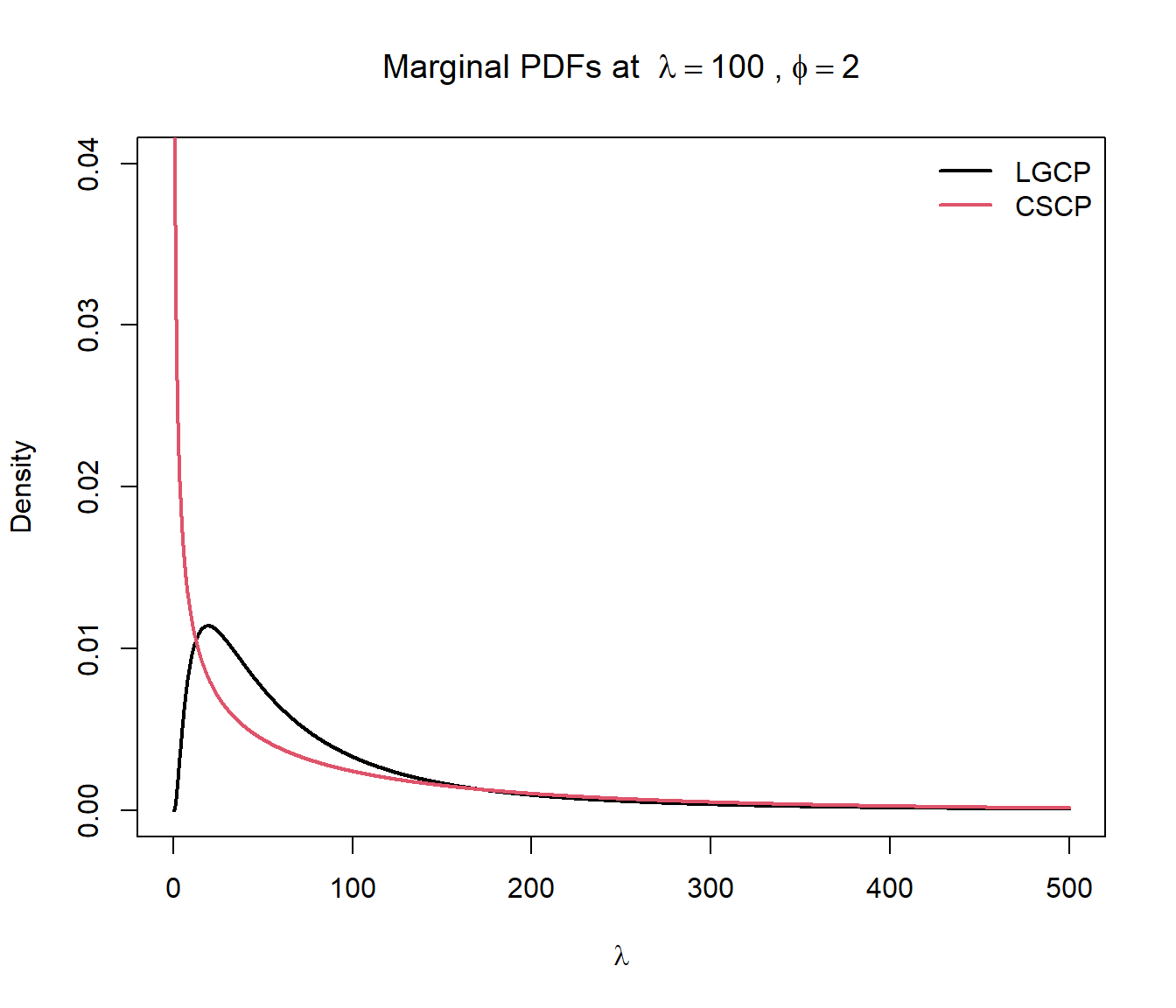
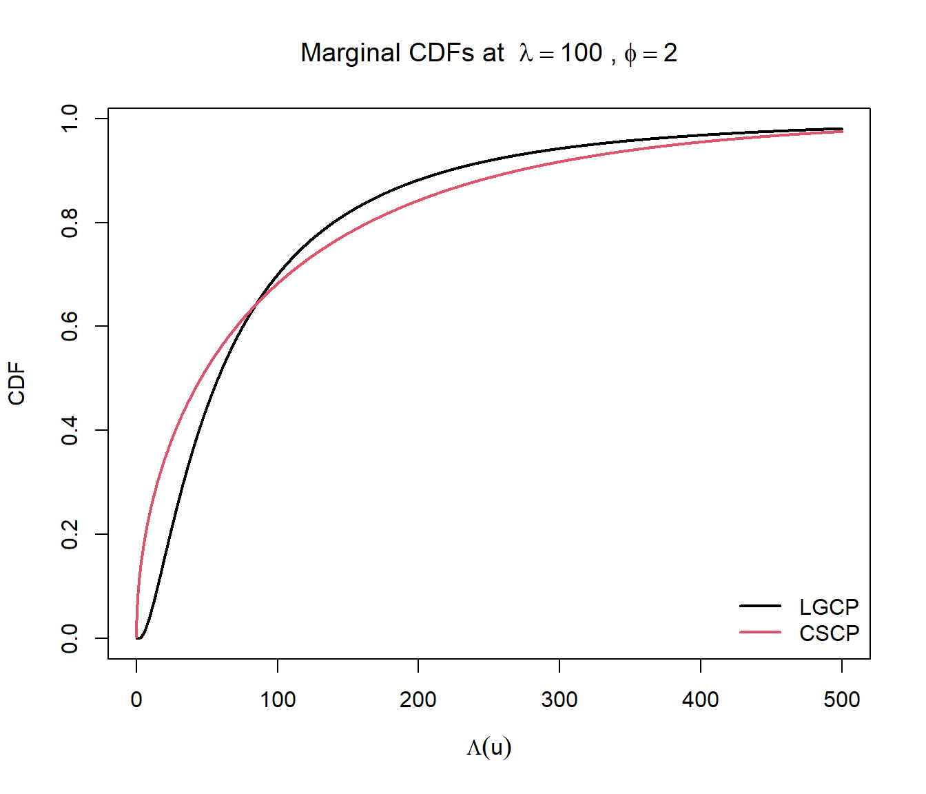
First we look at a single plot of the PDF with \((\lambda = 100, \phi = 2)\).
Several features are immediately apparent:
When \(\phi = 2\) (the maximum clustering strength under the CSCP parameterisation), the corresponding baseline shift parameter must satisfy \(\mu = 0\). In this case, the marginal distribution reduces exactly to a scaled \(\chi^2_1\) distribution.
Second interesting thing to note is that, for matched \((\lambda, \phi)\), the LGCP density is smoother and spreads probability mass more broadly across moderate intensity values, whereas the CSCP places more mass near its lower boundary due to the boundary singularity.
The CSCP density diverges as \(\lambda \to \mu^+\), reflecting a high concentration of probability mass near the lower bound.
Lastly, and I think the most important observation, is that the tails are, at least visually, on this scale, extremely similar. I was expecting at least a visible difference between the two, but they are almost indistinguishable.
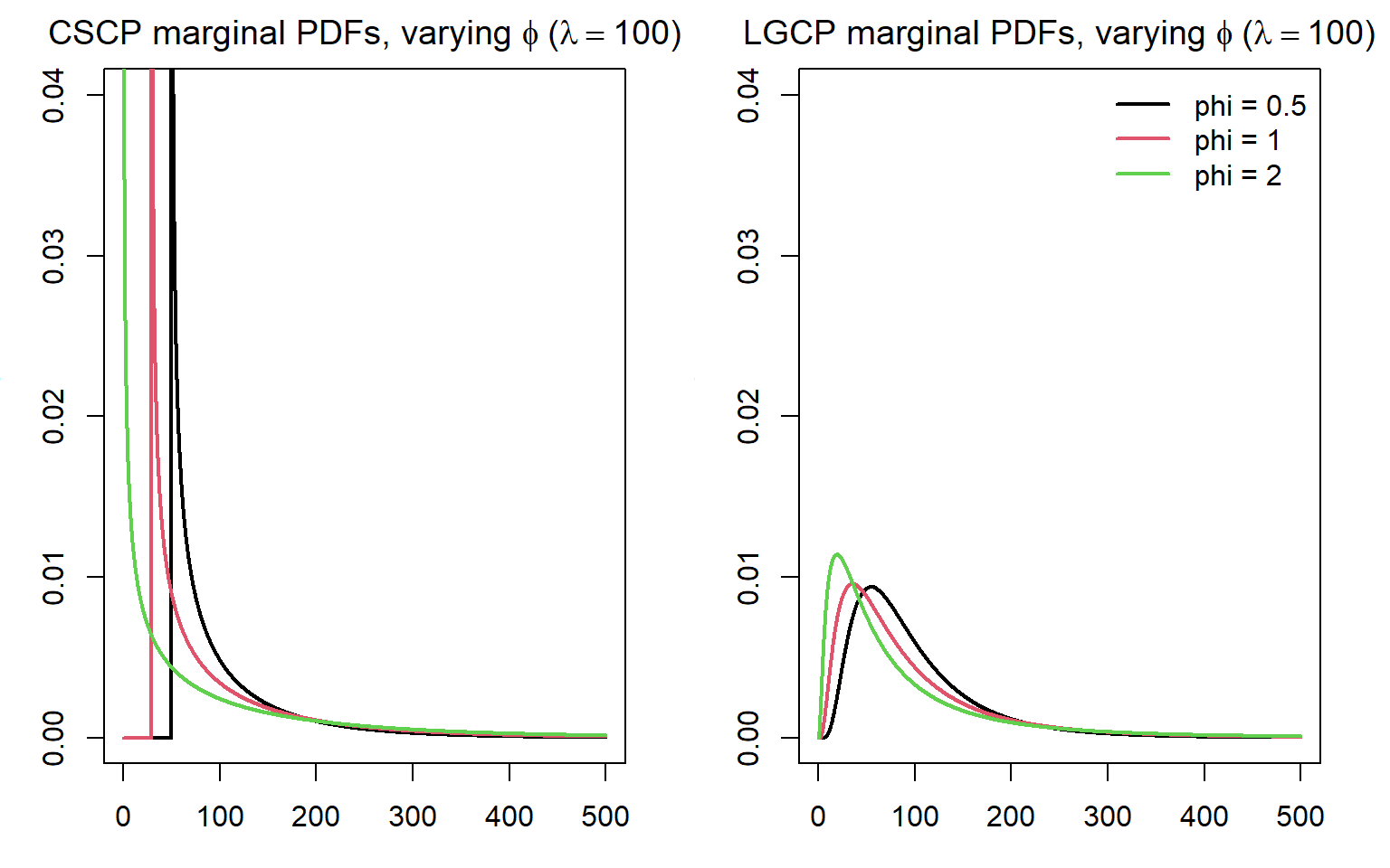
Effect of varying \(\phi\) on the PDFs
For the CSCP:
As \(\phi\) decreases, the lower bound \(\mu\) increases, and the concentration of mass near this boundary becomes less pronounced.
The overall shape of the density changes only moderately, with relatively subtle differences in curvature across values of \(\phi\).
For the LGCP:
As \(\phi\) decreases, the distribution becomes less dispersed, with more mass concentrated around moderate intensity values.
The peak of the density increases slightly, reflecting reduced variability in the latent field.
It is important to note that, under the LGCP parameterisation, the clustering strength \(\phi\) is determined by the variance \(\sigma^2\) of the underlying Gaussian field, and is independent of the mean parameter \(\mu\).
i
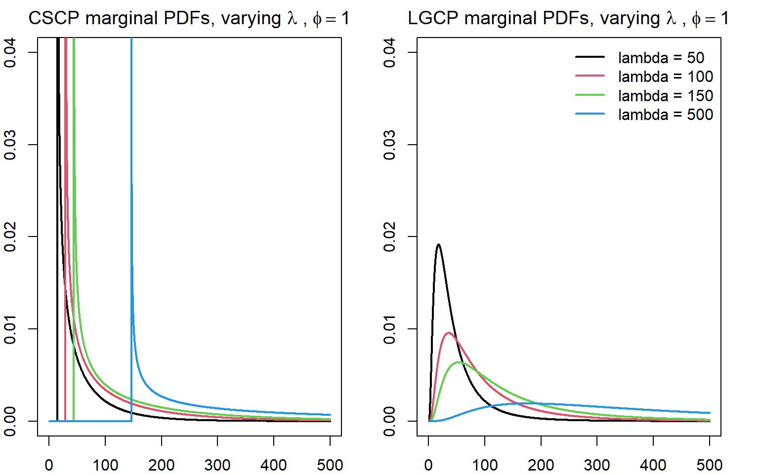
Effect of varying \(\lambda\) on the PDFs
For the CSCP:
Increasing \(\lambda\) primarily shifts the distribution, with relatively modest changes in shape. The behaviour near the lower bound remains a dominant feature across values of \(\lambda\).
For the LGCP:
As \(\lambda\) decreases, the distribution becomes more dispersed, with substantial probability mass extending over a wider range of intensities.
This reflects the interaction between the mean and variance parameters in the lognormal distribution, which jointly control both location and spread.
Note
Not super confident on the last bullet point there.
Note
What I believe is happening, is that the “heavier tails” of the LGCP mean that as \(\lambda\) increases, the PDF get “spread out” much faster than the CSCP.
To confirm this, it would be nice to have a clear way of seeing the \(\mu\) and \(\simga\) values for the LGCP and CSCP in the plot legends or something.
We might expect to see the rate of increase in \(\sigma\) relative to \(\lambda\), to be higher than that of the CSCP?
Suggested:
The apparent increase in spread for the LGCP as \(\lambda\) varies is driven by the interaction between the mean and variance of the underlying Gaussian field. Under the \((\lambda, \phi)\) parameterisation, changes in \(\lambda\) induce changes in both \(\mu\) and \(\sigma^2\), which together control the dispersion of the lognormal distribution.
This suggests that differences in variability between LGCP and CSCP marginals may be a useful feature for distinguishing the models.
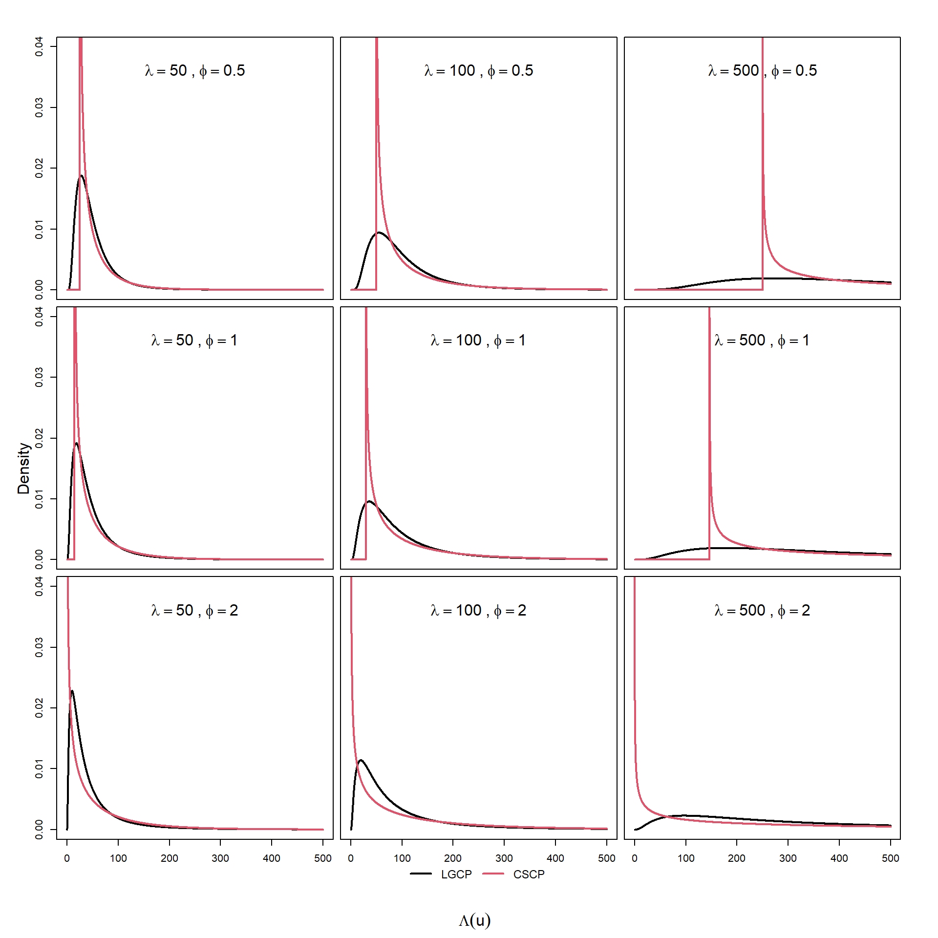
Taken together, these plots show that the LGCP and CSCP have structurally different marginal intensity distributions. The CSCP density has a hard lower bound and a boundary singularity, while the LGCP density is smoother near zero and more diffuse over moderate intensities.
Whether these differences are great enough to be detectable after the poisson thinning is yet to be seen.
To further investigate these differences, it is also useful to consider the corresponding cumulative distribution functions (CDFs), which may highlight differences in tail behaviour that are less apparent in the PDFs.
Note
I’m worried that the PDF is making the two marginal distributions look much more different than they really are.
44.4 CDFs
Corresponding cumulative distribution functions follow immediately from the transformed representations used above.
Note
I feel like it is slightly easier to think about how the marginal distribution might “effect” the observed patterns, by considering the CDF rather than PDF.
Additionally, as mentioned above, I think it is hard to gauge the mass is distributed from the PDF alone.
44.4.1 CSCP CDF
Recall that under the shifted CSCP,
\[
\Lambda(u) = \mu + Z(u)^2, \quad Z(u) \sim N(0, \sigma^2)
\] and from the previous subsection we showed that
So, at a fixed location \(u\), the marginal CDF of the LGCP is the CDF of a lognormal random variable.
44.4.3 Key differences
While the CSCP and LGCP can exhibit very similar second-order structure, their marginal cumulative distributions differ in important ways.
In particular:
Lower-tail behaviour:
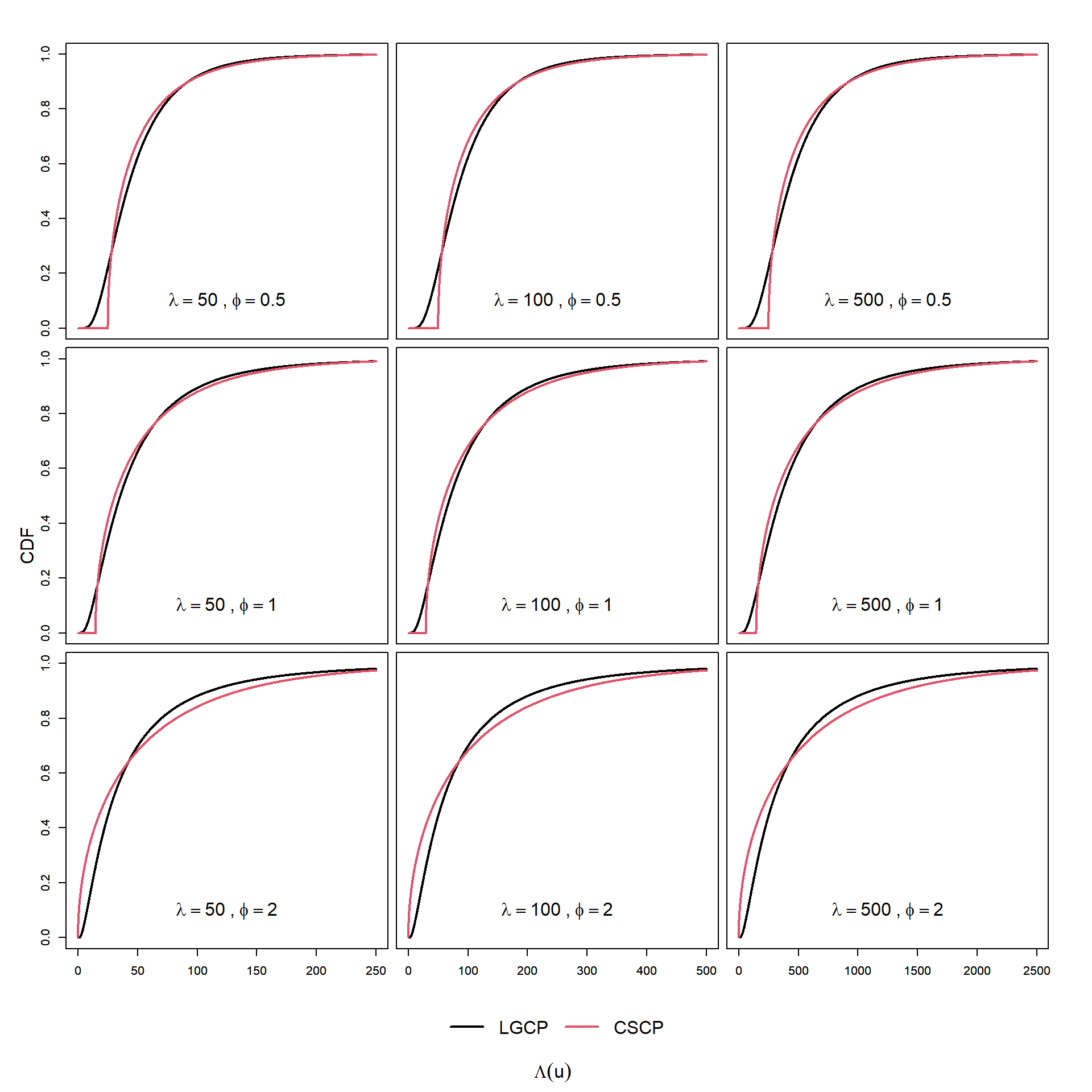
The CSCP CDF remains at zero up to the threshold \(\mu\), and then increases rapidly, reflecting a high concentration of probability mass near the lower bound. In contrast, the LGCP CDF increases smoothly from zero, indicating a more gradual accumulation of probability at low intensity levels.
Upper-tail behaviour:
The LGCP CDF approaches one more slowly, reflecting its heavier (lognormal) tail and greater probability of extreme intensity values. The CSCP CDF, by contrast, approaches one more rapidly due to its exponential tail decay.
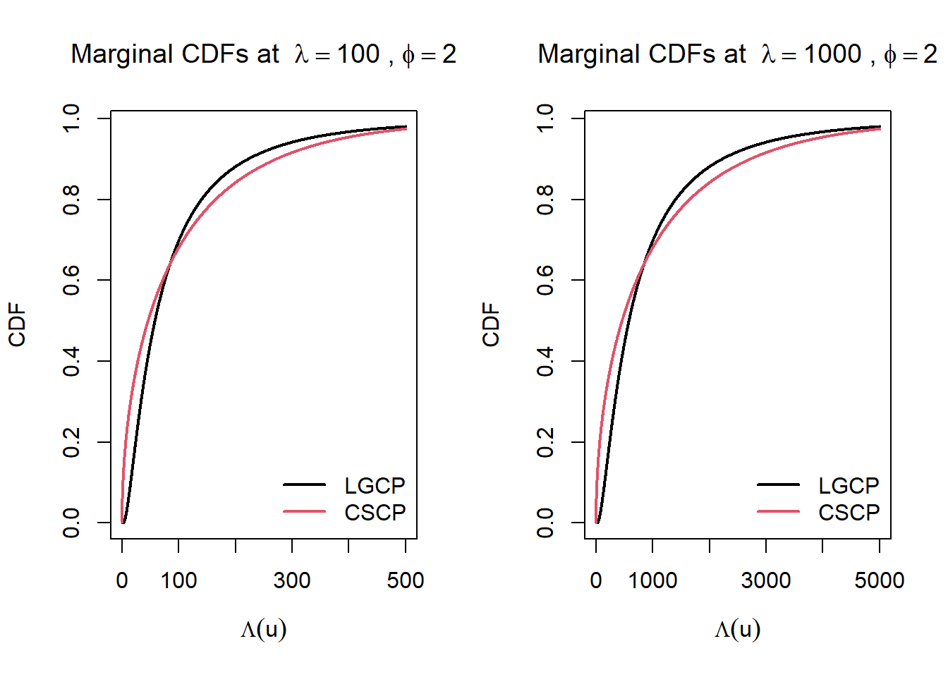
As in the PDF plots, when \(\phi = 2\) the CSCP CDF rises more rapidly at small values of \(\lambda\), reflecting a greater concentration of probability mass near the lower end of the marginal distribution.
This suggests that the CSCP may generate low-intensity regions more frequently than the LGCP. Through the Poisson sampling mechanism, this could in turn make small local counts or empty regions more likely, although this link is not direct and may be weakened in observed point patterns.
Note
Also, I believe this is he point I wanted to make earlier, regarding varying \(\lambda\) but keeping \(\phi\) fixed:
So, as demonstrated here, if we fix \(\phi\) and vary \(\lambda\), the the curves do not become more distinguishable (in the sense that the features do not change. Obviously, higher \(\lambda\) would mean more observed points and hence better classification).
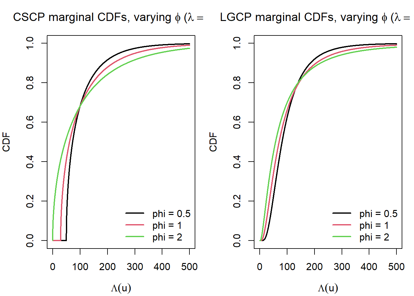
Varying \(\phi\), fixed \(\lambda\).
These plots show that changing \(\phi\) has a clear effect on the shape of the marginal CDFs under both models.
For the CSCP, larger values of \(\phi\) correspond to a stronger concentration of mass near the lower bound, leading to a sharper initial rise in the CDF.
For the LGCP, increasing \(\phi\) increases the spread of the lognormal distribution, which slows the accumulation of mass through the central region and leaves more probability in the upper tail.
As a result, the contrast between the two models is most pronounced at low thresholds, where the CSCP accumulates probability more rapidly.
Important
Notice that in the previous plots the PDFs of the LGCP and CSCP marginals appear very different, while the CDFs, while still different, appear much more similar.
This is a consequence of how the two summaries behave:
The PDF highlights local differences in density. Sharp features (such as spikes near zero or heavy tails) are clearly visible.
The CDF integrates these differences, effectively smoothing them out.
As a result, even when the underlying distributions differ substantially in shape, their cumulative behaviour can appear much closer.
From a statistical perspective, this suggests:
Differences in marginal distributions may be real, but not necessarily easy to detect using summaries that aggregate information, such as the CDF.
I believe this is the reason why, as we will see, it is so difficult to leverage these differences in an attempt to distinguish between the patterns.
Important
I want to add some kind of comment on why the CDF better reflects the summaries we actually observe from the data.
44.6 Comparing the tails
For the final part of this section, I focus on the upper tails of the LGCP and CSCP marginal distributions.
In particular, I want to investigate the LGCP’s heavier upper tail more directly. Although this is theoretically present, it is not especially easy to see from the density or distribution plots at ordinary plotting scales.
For a probability level \(p\), let \(q_p\) denote the upper quantile satisfying
\[
P(\Lambda(u) \le q_p) = p.
\]
Under each model, this is the value below which a proportion \(p\) of the marginal intensity distribution lies.
The tables below compare these upper-tail quantiles for the two models. The columns labelled “quantile / mean” express each quantile relative to the mean intensity \(\lambda\), so that, for example, a value of 3 means that the corresponding upper-tail quantile is three times the mean intensity.
The column “LGCP / CSCP quantile ratio” compares the two models directly: values larger than 1 indicate that the LGCP has the larger quantile at that probability level.
Upper-tail quantiles of the LGCP and CSCP marginal distributions, with \(\lambda = 100\) and \(\phi = 0.5\).
Quantile level
LGCP quantile
CSCP quantile
LGCP quantile / mean
CSCP quantile / mean
LGCP / CSCP quantile ratio
0.90000
184.6533
185.2772
1.84653
1.85277
0.99663
0.99000
359.1594
381.7448
3.59159
3.81745
0.94084
0.99900
584.1620
591.3783
5.84162
5.91378
0.98780
0.99990
871.8033
806.8353
8.71803
8.06835
1.08052
0.99999
1234.1720
1025.5711
12.34172
10.25571
1.20340
Upper-tail quantiles of the LGCP and CSCP marginal distributions, with \(\lambda = 100\) and \(\phi = 1\).
Quantile level
LGCP quantile
CSCP quantile
LGCP quantile / mean
CSCP quantile / mean
LGCP / CSCP quantile ratio
0.90000
205.5231
220.6001
2.05523
2.20600
0.93165
0.99000
490.4916
498.4474
4.90492
4.98447
0.98404
0.99900
926.4719
794.9139
9.26472
7.94914
1.16550
0.99990
1563.8108
1099.6160
15.63811
10.99616
1.42214
0.99999
2463.5313
1408.9551
24.63531
14.08955
1.74848
Upper-tail quantiles of the LGCP and CSCP marginal distributions, with \(\lambda = 100\) and \(\phi = 2\).
Quantile level
LGCP quantile
CSCP quantile
LGCP quantile / mean
CSCP quantile / mean
LGCP / CSCP quantile ratio
0.90000
221.2114
270.5543
2.21211
2.70554
0.81762
0.99000
661.3074
663.4897
6.61307
6.63490
0.99671
0.99900
1472.7431
1082.7566
14.72743
10.82757
1.36018
0.99990
2846.7700
1513.6705
28.46770
15.13671
1.88071
0.99999
5044.7171
1951.1421
50.44717
19.51142
2.58552
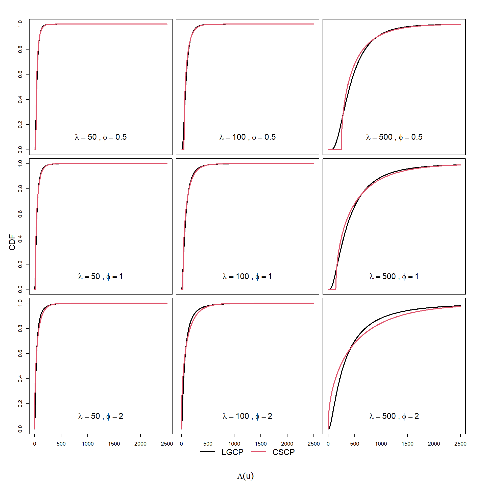
Across all values of \(\phi\), the same pattern is observed. At moderate quantile levels (up to around 0.99), the LGCP and CSCP marginal distributions are very similar, and in some cases the CSCP even produces slightly larger quantiles.
The difference between the models only becomes apparent in the extreme upper tail. Beyond the 0.999 quantile, the LGCP quantiles exceed those of the CSCP, and this gap increases rapidly as the quantile level increases. This effect is most pronounced for larger values of \(\phi\), where the LGCP can produce substantially more extreme intensity values.
Overall, while the LGCP does exhibit a heavier upper tail, this is primarily very-extreme-tail behaivour and is not visible in the bulk of the distribution.
44.7 Thoughts
Overall, the marginal distributions of the LGCP and CSCP differ in two key ways:
the CSCP places more mass near small intensity values, while the LGCP places relatively more mass over moderate values
the LGCP has a heavier upper tail, producing more extreme intensity values
However, the preceding analysis shows that these differences are not equally visible across all summaries.
In particular, while the PDFs highlight clear local differences in how mass is distributed, the CDFs appear much more similar, reflecting the fact that these differences are smoothed out when accumulated. This suggests that much of the distinction between the models is concentrated in relatively local features of the density, rather than in large global shifts of the distribution.
The tail analysis further reinforces this point. Although the LGCP does exhibit a heavier upper tail, this effect is primarily confined to very extreme quantiles, corresponding to rare events. At more moderate levels, the two models behave similarly, and in some cases the CSCP may even produce slightly larger quantiles.
Both effects present challenges for practical discrimination. The excess mass at small intensity values in the CSCP may be difficult to estimate reliably from observed data, as the underlying intensity surface is not directly observed. Similarly, the heavier tail of the LGCP manifests only in extreme events, which are unlikely to be well represented in finite samples.
Taken together, these results suggest that while the marginal distributions of the two models are theoretically distinct, the differences are subtle in a cumulative sense and may be difficult to exploit in practice.
This naturally raises the question of whether these marginal differences can be detected empirically from observed data.
In the next section, we investigate a naive approach to leveraging these differences.