par(mfrow = c(1, 2))
plot(longleaf)
plot(pcf(longleaf))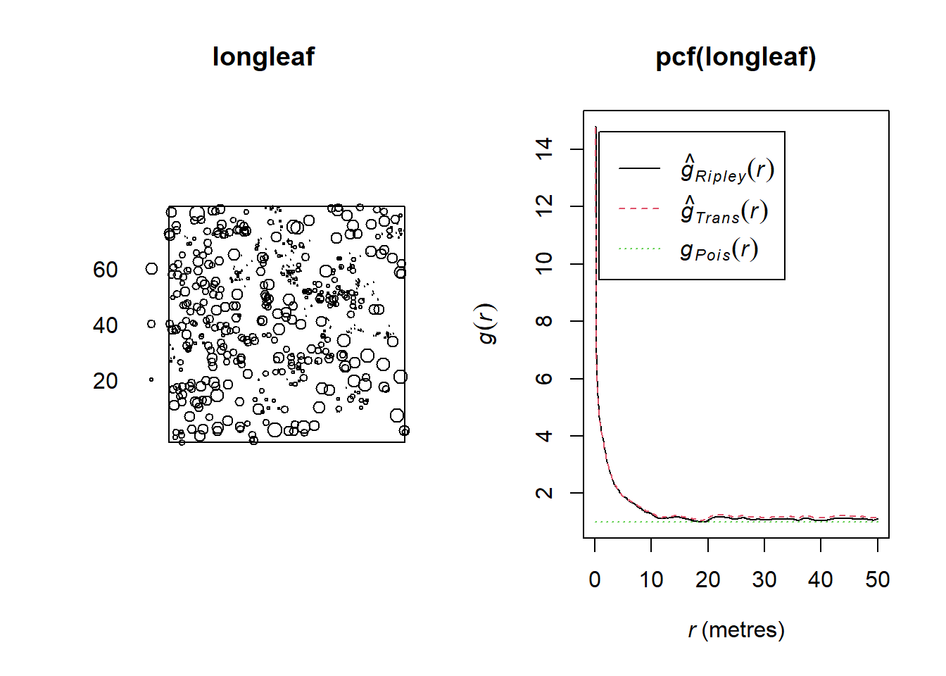
In the previous section, we introduced the second-order product density \(\lambda^{(2)}(u, v)\), which describes the joint occurrences of points at two locations.
However, this quantity is difficult to interpret directly:
To address this, we introduct a normalized version.
The pair correlation function (PCF) is defined as
\[ g(u, v) = \frac{\lambda^{(2)}(u, v)}{\lambda(u) \lambda(v)}, \quad u \neq v \] ## Interpretation
The PCF compares the observed joint occurrence of points at \(u\) and \(v\), to what would be expected under independence.
In particular:
\(g(u, v) = 1 \Longrightarrow\) no interaction (Poisson-like)
\(g(u, v) > 1 \Longrightarrow\) clustering (points occur together more often than expected)
\(g(u, v) > 1 \Longrightarrow\) repulsion (points inhibit each other)
The PCF removes the effect of intensity. It isolates the pure spatial ineraction between points.
For a Poisson process, we have:
\[ \lambda^{(2)}(u, v) = \lambda(u) \lambda(v) \]
and hence:
\[ g(u, v) = 1 \]
Thus, the PCF can be interpreted as a measure of deviation from complete spatial randomness.
Another useful way to interpret the PCF is:
\[ g(u,v) \approx \frac{\text{probability of observing a pair at } (u,v)} {\text{probability under independence}} \]
So:
\(g(u,v) = 2\) means that pairs occur twice as often as expected
\(g(u, v) = 0.5\) means that pairs occur half as often as expected
In many situations, interaction depends only on the distance between points.
In such cases, we write:
\[ r = \|u - v\| \]
and express the PCF as a function of distance, \(g(r)\).
This reduces the problem from studying interactions between all pairs of locations to understanding how interaction varies with separation distance.
This \(g(r)\) form is most commonly used in practice.
An example of a clustered process:
par(mfrow = c(1, 2))
plot(longleaf)
plot(pcf(longleaf))
And an example of a regular process:
par(mfrow = c(1, 2))
plot(hamster)
plot(pcf(hamster))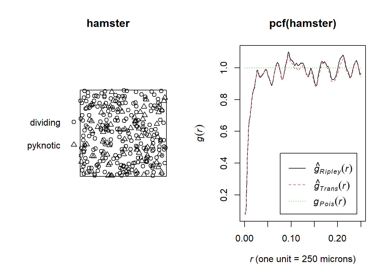
We now explore another second-order summary: the \(K\)-function, which aggregates interaction over distance and provides a complementary perspective.