50 Minimum contrast

I’ve implemented my own minimum contrast. You can find the code here

50.1 Examples

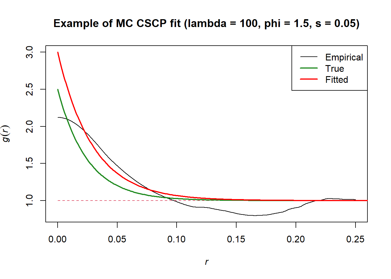
Fitting a CSCP minimum contrast model:

Code

set.seed(1)
# Simulating a point pattern realization from a CSCP on window [0,1]x[0,1] 
cscp_pp <- sim_cscp(lambda = 100, phi = 1.5, s = 0.05)$pp

# Fitting a MC model
cscp_fit <- fit_cscp_mc(cscp_pp, bw = 0.02)

# Comparing the model fit to the true PCF
r_vals <- seq(0, 2.5, by = 0.001)

fitted_pcf_vals <- pcf_cscp_theoretical(r_vals, lambda = cscp_fit$par[["lambda"]], 
                                        phi = cscp_fit$par[["phi"]], 
                                        s = cscp_fit$par[["s"]])
theoretical_pcf_vals <- pcf_cscp_theoretical(r_vals, lambda = 100, phi = 1.5, s = 0.05)

plot(pcf(cscp_pp, correction = "isotropic", divisor = "a",
                        zerocor = "JonesFoster", bw = 0.02), 
     ylim = c(0.8, 3), legend = F, main = "Example of MC CSCP fit (lambda = 100, phi = 1.5, s = 0.05)")
lines(r_vals, theoretical_pcf_vals, col = "forestgreen", lwd = 2)
lines(r_vals, fitted_pcf_vals, col = "red", lwd = 2)
legend("topright", legend = c("Empirical", "True", "Fitted"), col = c("black", "forestgreen", "red"), lwd = c(1, 2, 2))

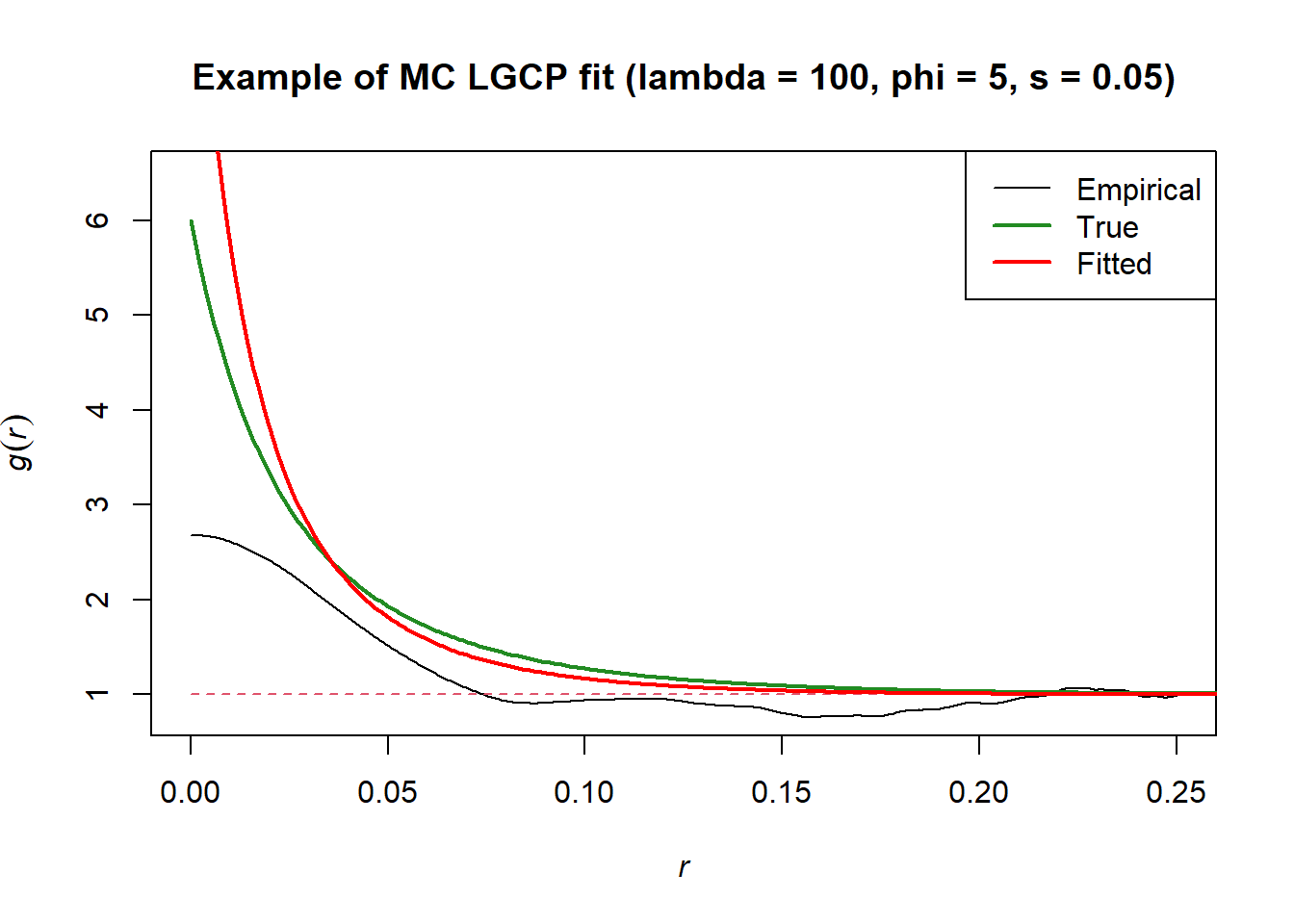
Fitting an LGCP minimum contrast model:

Code

set.seed(1)
# Simulating a point pattern realization from a CSCP on window [0,1]x[0,1] 
lgcp_pp <- sim_lgcp(lambda = 100, phi = 5, s = 0.05)$pp

# Fitting a MC model
# Notice we have used a smaller bandwidth for this fit
lgcp_fit <- fit_lgcp_mc(lgcp_pp, bw = 0.01)

# Comparing the model fit to the true PCF
r_vals <- seq(0, 1, by = 0.001)

fitted_pcf_vals <- pcf_lgcp_theoretical(r_vals, lambda = lgcp_fit$par[["lambda"]], 
                                        phi = lgcp_fit$par[["phi"]], 
                                        s = lgcp_fit$par[["s"]])
theoretical_pcf_vals <- pcf_lgcp_theoretical(r_vals, lambda = 100, phi = 5, s = 0.05)

plot(pcf(cscp_pp, correction = "isotropic", divisor = "a",
                        zerocor = "JonesFoster", bw = 0.01), 
     ylim = c(0.8, 6.5), legend = F, main = "Example of MC LGCP fit (lambda = 100, phi = 5, s = 0.05)")
lines(r_vals, theoretical_pcf_vals, col = "forestgreen", lwd = 2)
lines(r_vals, fitted_pcf_vals, col = "red", lwd = 2)
legend("topright", legend = c("Empirical", "True", "Fitted"), col = c("black", "forestgreen", "red"), lwd = c(1, 2, 2))

50.2 Implementation notes

Firstly, spatstat already provides a very useful mincontrast() function, and it is probably faster and more reliable than my implementation, but if I didn’t do this I would never bother to understand what is happening under the hood. I would eventually like to implement the non-parameteric PCF estimators as well.

I will comment on the CSCP implementation below, the LGCP is almost the same. I’ve left the in-line documentation out here, see the source file linked above if you prefer reading that, or use ?fit_cscp_mc after loading the library.

Code

estimate_pcf_for_mc <- function(X,
                                bw = 0.2,
                                correction = "isotropic",
                                divisor = "a",
                                zerocor = "JonesFoster",
                                r_min = 0.02,
                                r_max = NULL) {
  stopifnot(inherits(X, "ppp"))

  obs <- spatstat.explore::pcf(
    X,
    bw = bw,
    correction = correction,
    divisor = divisor,
    zerocor = zerocor
  )

  y_name <- switch(
    correction,
    isotropic = "iso",
    translate = "trans",
    Ripley = "iso",
    "iso"
  )

  if (!y_name %in% names(obs)) {
    y_name <- intersect(c("iso", "trans", "un"), names(obs))[1]
  }

  r <- obs$r
  g <- obs[[y_name]]

  keep <- is.finite(r) & is.finite(g) & r > r_min
  if (!is.null(r_max)) keep <- keep & r <= r_max

  list(
    fv = obs,
    r = r[keep],
    g = g[keep],
    correction_used = y_name,
    bw = bw,
    divisor = divisor,
    zerocor = zerocor,
    r_min = r_min,
    r_max = r_max
  )
}

mc_pcf_objective <- function(par,
                             r,
                             g_obs,
                             model = c("lgcp", "cscp"),
                             lambda,
                             df = 1,
                             k = 0.25,
                             p = 2) {
  model <- match.arg(model)

  if (model == "lgcp") {
    phi <- exp(par[1]) # phi in (0, Inf)              
    s   <- exp(par[2]) # s > 0              
    g_th <- pcf_lgcp_theoretical(
      r,
      lambda = lambda,
      phi = phi,
      s = s
    )
  } else {
    # Note for CSCP we need to transform the parameters in order to
    # use the pcf_cscp_theoretical() function.
    eta <- par[1] # eta in R                   
    phi <- 2 * stats::plogis(eta) # phi in (0, 2)   
    s   <- exp(par[2]) # s > 0              
    g_th <- pcf_cscp_theoretical(
      r,
      lambda = lambda,
      phi = phi,
      s = s,
      df = df
    )
  }

  sum(abs(g_obs^k - g_th^k)^p)
}

fit_cscp_mc <- function(X,
                        start = list(phi = 0.5, s = 0.05),
                        df = 1,
                        bw = 0.2,
                        correction = "isotropic",
                        divisor = "a",
                        zerocor = "JonesFoster",
                        r_min = 0.02,
                        r_max = NULL,
                        k = 0.25,
                        p = 2) {
  stopifnot(inherits(X, "ppp"))
  stopifnot(is.list(start), !is.null(start$phi), !is.null(start$s))
  stopifnot(start$phi > 0, start$phi < 2, start$s > 0)

  lambda_hat <- spatstat.geom::intensity(X)

  pcf_obs <- estimate_pcf_for_mc(
    X,
    bw = bw,
    correction = correction,
    divisor = divisor,
    zerocor = zerocor,
    r_min = r_min,
    r_max = r_max
  )

  # Inverse of phi = 2*plogis(eta)
  eta_start <- stats::qlogis(start$phi / 2)

  opt <- stats::optim(
    par = c(eta_start, log(start$s)),
    fn = mc_pcf_objective,
    r = pcf_obs$r,
    g_obs = pcf_obs$g,
    model = "cscp",
    lambda = lambda_hat,
    df = df,
    k = k,
    p = p,
    method = "L-BFGS-B",
    lower = c(-20, log(1e-8)),
    upper = c(20, log(10))
  )

  pars <- c(
    lambda = lambda_hat,
    phi = 2 * stats::plogis(opt$par[1]),
    s = exp(opt$par[2])
  )

  g_fit <- pcf_cscp_theoretical(
    pcf_obs$r,
    lambda = pars["lambda"],
    phi = pars["phi"],
    s = pars["s"],
    df = df
  )

  structure(
    list(
      model = "CSCP",
      df = df,
      par = pars,
      objective = opt$value,
      convergence = opt$convergence,
      optim = opt,
      eta_hat = opt$par[1],
      r = pcf_obs$r,
      g_obs = pcf_obs$g,
      g_fit = g_fit,
      pcf_obs = pcf_obs
    ),
    class = "mc_pcf_fit"
  )
}

Basic structure

The fitting routine proceeds as follows:

Compute an empirical pair correlation function using estimate_pcf_for_mc().
Estimate the intensity $\lambda$ from the observed point pattern using spatstat.geom::intensity(X).
Convert the user-supplied starting value for $\phi$ into the unconstrained parameter $\eta$.
Minimize the minimum contrast objective using optim().
Back-transform the optimized parameters to the original scale and return both the fitted parameters and fitted PCF values.

Note $\lambda$ is not optimized within the minimum contrast step.

The objective function is:

\[ \sum_i |\hat{g}(r_i)^k - g(r_i; \theta)^k|^p, \]

where $\hat{g}(r_i)$ is the empirical PCF, $g(r_i; \theta)$ is the theoretical PCF under the model, and $k$ and $p$ are tuning constants.

Reparameterization from $\phi$ to $\eta$

In the case of the CSCP, the parameter space of $\phi$ is $[0, 2]$, and of $s$ is $[0, \infty)$.

To enforce $\phi \in [0, 2]$, we optimize over $\eta$, where $\phi = 2\cdot \text{plogis}(\eta)$.

To enforce $s \in [0, \infty)$, we optimize over $\log(s)$.

Default values

I chose the following as default values, with my justification being they either produced fairly decent fits in my limited experience, or because they were suggested by my GOATs (supervisors).

Argument	Default	Role
`bw`	`0.2`	Bandwidth for empirical PCF estimation
`correction`	`"isotropic"`	Edge correction used in `pcf()`
`divisor`	`"a"`	Denominator choice for `pcf()`
`zerocor`	`"JonesFoster"`	Correction near the origin
`r_min`	`0.02`	Lower cutoff for fitting range
`r_max`	`NULL`	Upper cutoff for fitting range
`k`	`0.25`	Power transform in minimum contrast
`p`	`2`	Loss power
`start$phi`	`0.5`	Starting value for clustering strength
`start$s`	`0.05`	Starting value for range/scale

I also understand the argument for using whatever spatstat uses as its defaults.

Criticsms

It’s a pain in the ass to plot the fitted vs empirical right now. Would be nice to be able to streamline this.
Also, The way I have it setup right now is not very flexible if we want to consider different models in the future. In particular, a better design pattern might have been to have users pass there own objective function, rather than the way I have mc_pcf_objective() used internally (spatstat has the users pass it to mincontrast()).
I also think spatstat fits minimum contrast by using the K-function by default? Maybe this would be better.
I don’t really know the theory behind the $k$ and $p$ tuning parameters.

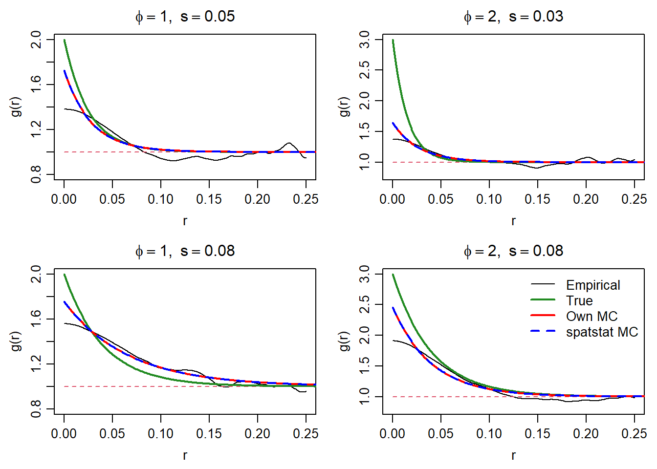
50.3 Comparison to `spatstat` implementation

THANK frick they are (almost) identical. I can rest in peace.

50.4 Todo

Add inline & roxygen comments.
I hate how annoying it is to plot the fitted PCF vs observed. Will be implementing a class + summary / plotting methods.
It would be nice if we could calculate the empirical PCF using spatstat’s PCF function, and then just pass that PCF object to the minimum contrast fitting function we have. Makes comparing different fits easier, and feels more reliable.
I have no idea above uncertainty quantification for MC fitting. Will look into this.
I believe the reparameterization of $\phi$ to $\eta$ does not allow estimates of $\phi \in \{0, 1\}$. Is this a problem?

50.1 Examples

50.2 Implementation notes

50.3 Comparison to spatstat implementation

50.4 Todo

50.3 Comparison to `spatstat` implementation