38  Second-order Structure Comparison to LGCPs

An important question we have been investigating is whether a point pattern generated by a chi-square Cox process (CSCP) can be distinguished from one generated by a log-Gaussian Cox process (LGCP) (single component).

Since the two models arise from different latent constructions, we might expect them to produce visibly different realizations. A natural place to begin then, is with a simple visual comparison: are the differences between the two processes large enough that they can be noticed directly from their intensity surfaces or point patterns?

Note

Will make these nicer later, SO annoying trying to get them to play nice, I actually despise the default plotting from spatstat.

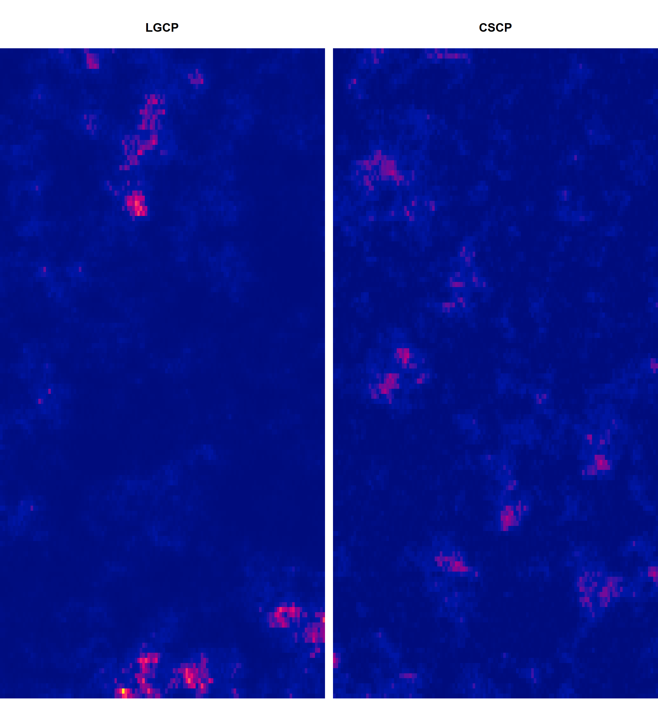
When the parameters are matched exactly, the two processes appear slightly different upon visual inspection of their intensity surfaces (and less so from the resulting point patterns).

Now obviously visual inspection alone is not sufficient for model comparison in practice. Instead, it is common to rely on second-order summary statistics, such as the pair correlation function (PCF), which capture the dependence structure of the process.

We therefore turn our attention towards a comparison of the theoretical PCFs of the two models.

Consider the following plot of 2 processes (LGCP and CSCP), on a \([0, 1]\times[0, 1]\) window:

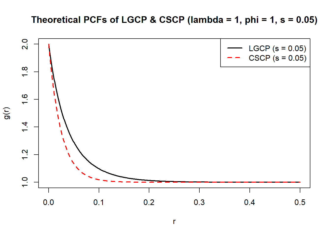
The two pair correlation functions are clearly different when all parameters are matched.

However, this comparison is somewhat artificial.

In practice, we obviously do not know the true parameters of the models, and must estimate them from the observed point pattern. When fitting competing models, each model is free to select parameter values that best reproduce the observed structure.

As a result, even if two models differ under identical parameter values, they may still produce very similar second-order behaviour after fitting.

Importantly, while the parameters \(\lambda\) and \(\phi = g(0) - 1\) have a common interpretation across both models, controlling the overall intensity and the strength of clustering at the origin, the scale parameter \(s\) plays a more subtle role.

In the LGCP, \(s\) governs the decay of correlation in the latent Gaussian field, and leads to a PCF of the form

\[ g(r) = \exp\big(\sigma^2 \exp(-r/s)\big), \]

whereas in the CSCP, the dependence arises through squared Gaussian fields, resulting in

\[ g(r) = 1 + \phi \exp(-2r/s). \]

Thus, although both parameters are referred to as “scale”, they do not represent the same structural feature, and equating them does not lead to a meaningful comparison of the models.

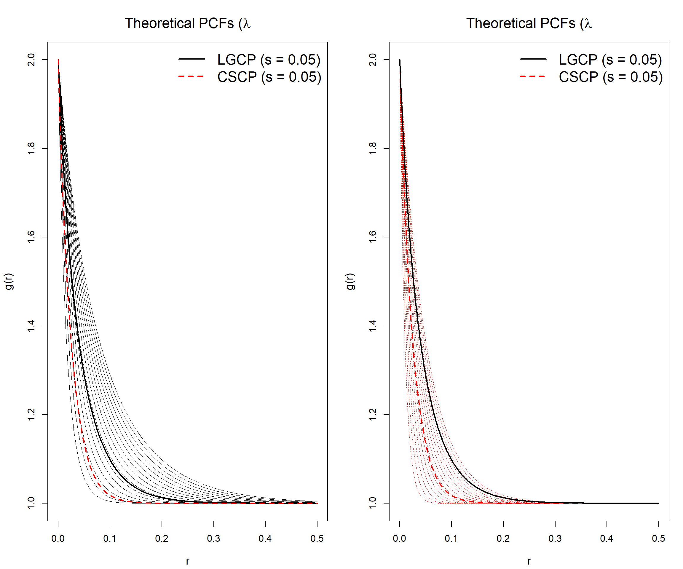
This suggests a more appropriate comparison: fix the first-order intensity \(\lambda\) and clustering strength \(\phi\), and allow the scale parameter to vary. This reflects the practical setting in which models are fitted to data.

The following plots demonstrate that, under this setup, an LGCP can closely approximate the PCF of a CSCP by suitably adjusting its scale parameter (and vice versa).

Note

Title clipping, will fix later.

And consider a single example, demonstrating a good approximation of LGCP PCF with scale = 0.05 by a CSCP PCF with scale = 0.085.

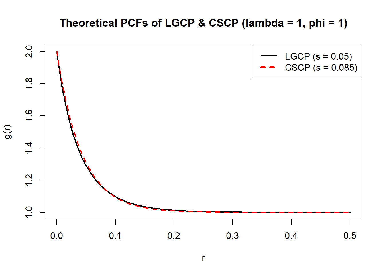
Even after fixing first-order intensity and clustering strength, the models retain enough flexibility through their scale parameter to closely match each other’s pair correlation functions.

This suggests that the two models may be difficult to distinguish based on second-order structure alone, even though they arise from fundamentally different constructions.

This motivates the central question of this chapter:

To what extent are LGCPs and CSCPs identifiable from their pair correlation functions?

and perhaps in the future:

What aspects of the models (if any) allow them to be distinguished in practice?