41  🚧 Empirical comparison of PCF families

41.1 Numerical optimisation

To study the approximation problem, we numerically solve

\[ p^*(\phi) \in \arg \min_{p > 0} \sup_{x \in [0,1]} \left| \exp(c x^p) - 1 - \phi x \right|, \quad c = \log(1 + \phi), \]

for values of \(\phi \in [0,2]\).

The supremum over \(x\) is approximated using a fine grid over \([0,1]\), and the minimisation over \(p\) is carried out using one-dimensional optimisation.

Code:

# Shouldve just used my package functions, but was still under construction
g_cscp <- function(r, phi, s_C) {
  1 + phi * exp(-2 * r / s_C)
}

g_lgcp <- function(r, phi, s_L) {
  (1 + phi)^(exp(-r / s_L))
}

# E(phi, p) = sup_{x in [0,1]} | exp(c x^p) - 1 - phi x |
pcf_error_p <- function(phi, p, x_grid = seq(0, 1, length.out = 4000)) {
  cval <- log(1 + phi)
  max(abs(exp(cval * x_grid^p) - 1 - phi * x_grid))
}

# same thing, but using a scale ratio alpha = s_L / s_C
pcf_error_alpha <- function(phi, alpha, x_grid = seq(0, 1, length.out = 4000)) {
  p <- 1 / (2 * alpha)
  pcf_error_p(phi, p, x_grid = x_grid)
}

# Slope matching - intially thought I would include as a 
# "rule-of-thumb" type thing, but it's too shitty to keep tbh
alpha_slope <- function(phi) {
  ifelse(phi == 0, 1/2, ((1 + phi) * log(1 + phi)) / (2 * phi))
}

p_slope <- function(phi) {
  1 / (2 * alpha_slope(phi))
}

find_optimal_match <- function(phi,
                               x_grid = seq(0, 1, length.out = 4000),
                               alpha_lower = 0.05,
                               alpha_upper = 5) {
  
  obj_alpha <- function(alpha) {
    pcf_error_alpha(phi, alpha, x_grid = x_grid)
  }
  
  opt <- optimize(obj_alpha, interval = c(alpha_lower, alpha_upper))
  
  alpha_opt <- opt$minimum
  err_opt   <- opt$objective
  alpha_h   <- alpha_slope(phi)
  err_h     <- obj_alpha(alpha_h)
  
  tibble(
    phi = phi,
    alpha_opt = alpha_opt,
    alpha_slope = alpha_h,
    p_opt = 1 / (2 * alpha_opt),
    p_slope = p_slope(phi),
    err_opt = err_opt,
    err_slope = err_h
  )
}

41.2 Optimal scale relationship

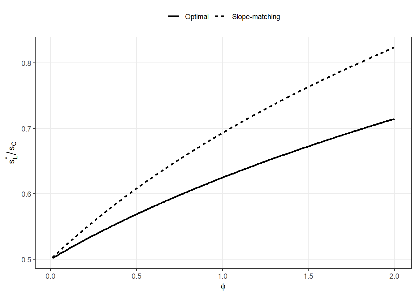
We first examine how the optimal LGCP scale relates to the CSCP scale.

Define the scale ratio

\[ \alpha^*(\phi) = \frac{s_L^*(\phi)}{s_C}. \]

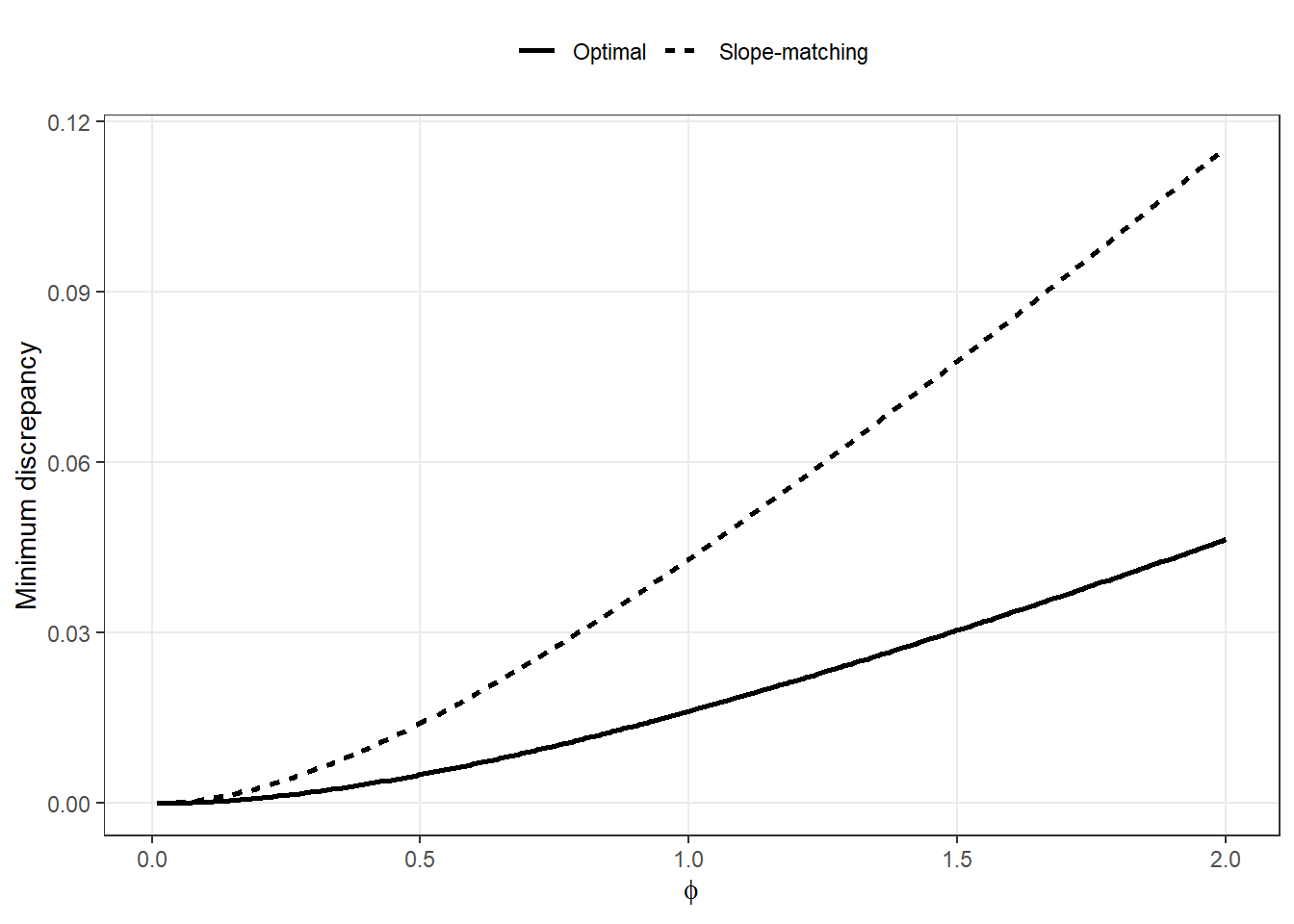
The figure below shows \(\alpha^*(\phi)\) as a function of \(\phi\), along with the slope-matching approximation

\[ \alpha_{\text{slope}}(\phi) = \frac{(1+\phi)\log(1+\phi)}{2\phi}. \]

Note

Originally, I wanted to have some sort of closed-form approximation of the best approximating ratio for a given \(\phi\), but it seems less useful than just making a function which numerically calculates it for you basically instantly.

phi_grid <- seq(0.01, 2, length.out = 200)

opt_results <- map_dfr(phi_grid, find_optimal_match)

# opt_results
scale_plot_df <- opt_results %>%
  select(phi, alpha_opt, alpha_slope) %>%
  pivot_longer(cols = c(alpha_opt, alpha_slope),
               names_to = "method",
               values_to = "alpha")

scale_plot_df$method <- factor(
  scale_plot_df$method,
  levels = c("alpha_opt", "alpha_slope"),
  labels = c("Optimal", "Slope-matching")
)

ggplot(scale_plot_df, aes(x = phi, y = alpha, linetype = method)) +
  geom_line(linewidth = 0.9) +
  labs(
    x = expression(phi),
    y = expression(s[L]^"*" / s[C]),
    linetype = NULL
  ) +
  theme_bw() +
  theme(
    legend.position = "top",
    panel.grid.minor = element_blank()
  )

41.3 Approximation error

We now examine the minimum discrepancy:

\[ E^*(\phi) := \inf_{p > 0} \sup_{x \in [0,1]} \left| \exp(c x^p) - 1 - \phi x \right| \]

The figure below shows \(E^*(\phi)\) as a function of \(\phi\), along with the discrepancy obtained using the slope-matching approximation.

err_plot_df <- opt_results %>%
  select(phi, err_opt, err_slope) %>%
  pivot_longer(cols = c(err_opt, err_slope),
               names_to = "method",
               values_to = "error")

err_plot_df$method <- factor(
  err_plot_df$method,
  levels = c("err_opt", "err_slope"),
  labels = c("Optimal", "Slope-matching")
)

ggplot(err_plot_df, aes(x = phi, y = error, linetype = method)) +
  geom_line(linewidth = 0.9) +
  labs(
    x = expression(phi),
    y = "Minimum discrepancy",
    linetype = NULL
  ) +
  theme_bw() +
  theme(
    legend.position = "top",
    panel.grid.minor = element_blank()
  )

Note

Might be nice to replot this as some type of error relative to the curves.

For example, maybe relative to the current height of the curve above 1?

41.4 Visual comparison of PCFs

To better understand the approximation, we compare the PCF curves directly for selected values of \(\phi\).

In each panel we show:

• the CSCP PCF (solid line)

• the best-fitting LGCP PCF (dashed line)

phi_panel <- c(0.1, 0.8, 1.5, 2.0)
s_C_fixed <- 1
r_grid <- seq(0, 4, length.out = 1000)

panel_match <- map_dfr(phi_panel, find_optimal_match)

pcf_panel_df <- map_dfr(seq_along(phi_panel), function(i) {
  phi_i <- phi_panel[i]
  alpha_i <- panel_match$alpha_opt[panel_match$phi == phi_i]
  s_L_i <- alpha_i * s_C_fixed
  
  tibble(
    r = rep(r_grid, 2),
    g = c(
      g_cscp(r_grid, phi = phi_i, s_C = s_C_fixed),
      g_lgcp(r_grid, phi = phi_i, s_L = s_L_i)
    ),
    model = rep(c("CSCP", "Best LGCP"), each = length(r_grid)),
    phi_lab = paste0("phi = ", phi_i)
  )
})

ggplot(pcf_panel_df, aes(x = r, y = g, colour = model, linetype = model)) +
  geom_line(linewidth = 0.9) +
  facet_wrap(~ phi_lab, ncol = 2, scales = "fixed") +
  labs(
    x = "r",
    y = "PCF",
    colour = NULL,
    linetype = NULL
  ) +
  theme_minimal() +
  theme(
    legend.position = "top",
    panel.grid.minor = element_blank()
  )

41.5 Sampling variability vs model difference

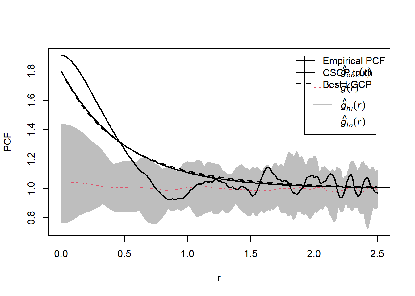
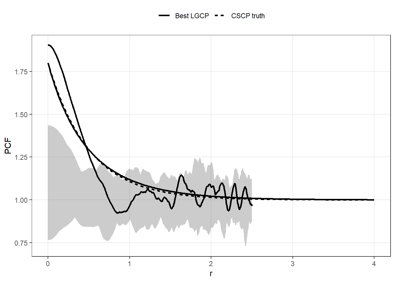
To assess whether the two models can be distinguished in practice, we compare the difference between the PCF curves to the sampling variability of the PCF estimator.

We:

• simulate a CSCP point pattern,
• estimate the PCF,
• construct simulation envelopes,
• and overlay the true CSCP PCF and the best-fitting LGCP PCF.

Note

Not finished, but you get the idea of what I’m trying to show here, right?

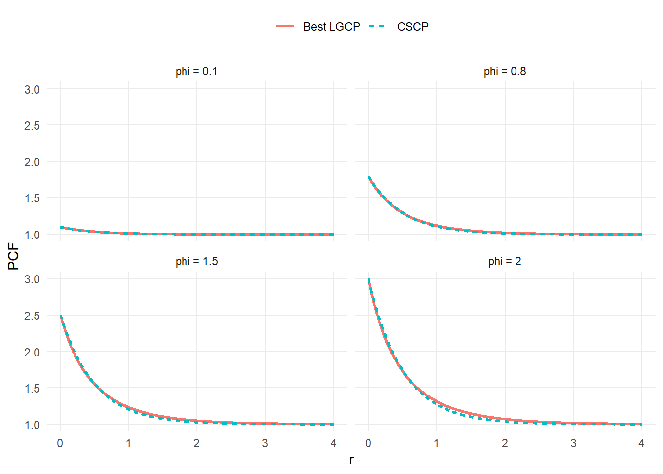
41.6 Interpretation

Across all values of \(\phi\), the discrepancy between the LGCP and CSCP PCFs can be made very small by appropriately rescaling the LGCP.

Moreover, the difference between the two PCF curves is typically small relative to the sampling variability of standard PCF estimators.

This suggests that, in practice, the two models are difficult to distinguish based on second-order structure alone.

41.7 What’s next?

So far we have shown:

• The PCFs of the LGCP and CSCP can approximate each other closely, and
  
• The differences between the two families are small relative to the sampling variability of standard PCF estimators.

This is nice, however what we would like to claim is:

• Procedures based on second-order summaries, such as minimum contrast estimation, lead to similar conclusions under LGCP and CSCP models.

The next section investigates this empirically by fitting each models to data generated by both LGCPs and CSCPs, and compares the resulting fits and parameter estimates.

41.8 Extras

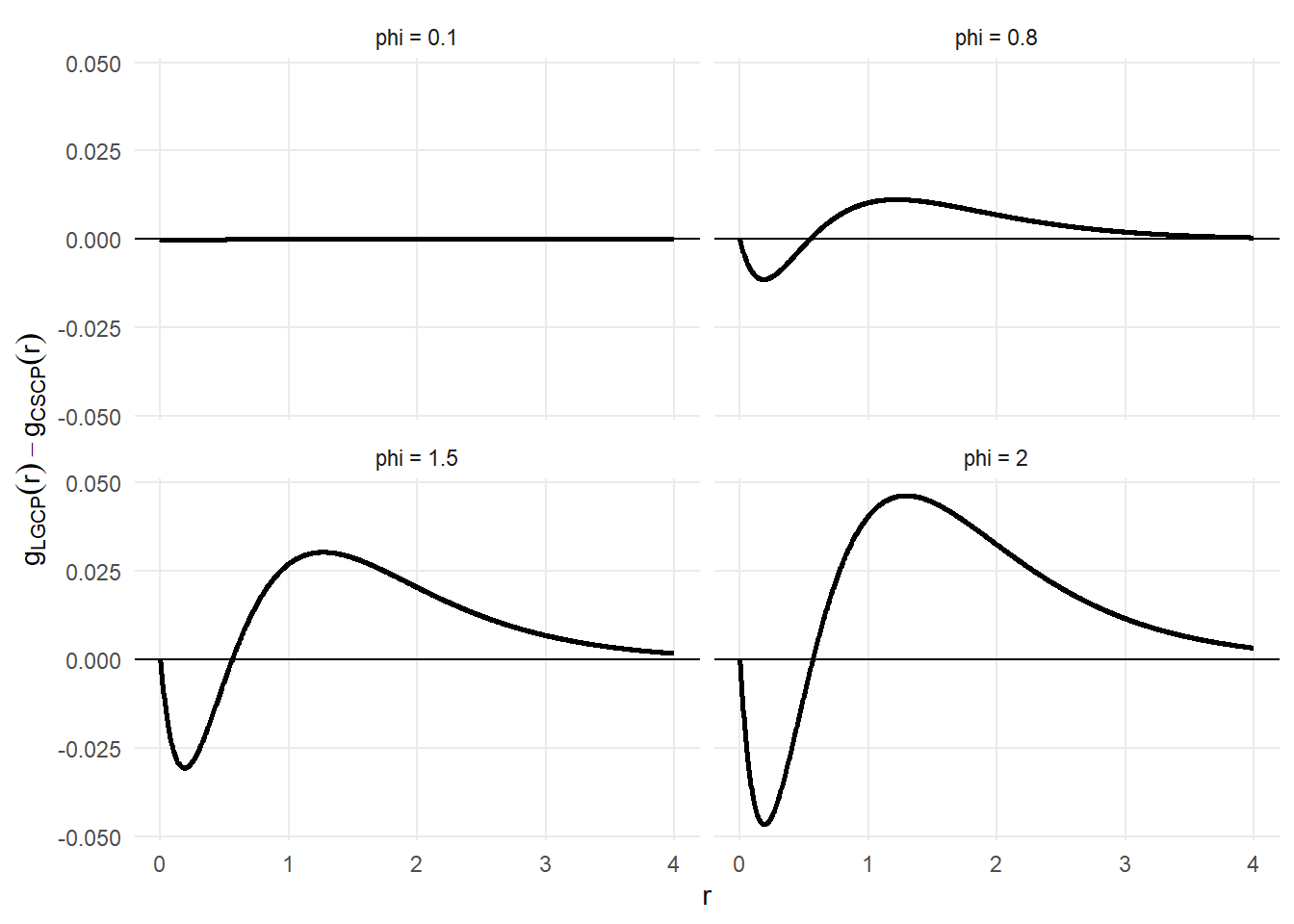
41.8.1 Difference between PCFs

To highlight where the two models differ, we plot

\[ g_{LGCP}(r) - g_{CSCP}(r) \]

for selected values of \(\phi\).

This is looking at how different the two curves are as we increase \(r\).

diff_df <- map_dfr(seq_along(phi_panel), function(i) {
  phi_i <- phi_panel[i]
  alpha_i <- panel_match$alpha_opt[panel_match$phi == phi_i]
  s_L_i <- alpha_i * s_C_fixed
  
  tibble(
    r = r_grid,
    diff = g_lgcp(r_grid, phi = phi_i, s_L = s_L_i) -
      g_cscp(r_grid, phi = phi_i, s_C = s_C_fixed),
    phi_lab = paste0("phi = ", phi_i)
  )
})

ggplot(diff_df, aes(x = r, y = diff)) +
  geom_hline(yintercept = 0, linewidth = 0.4) +
  geom_line(linewidth = 0.9) +
  facet_wrap(~ phi_lab, ncol = 2, scales = "fixed") +
  labs(
    x = "r",
    y = expression(g[LGCP](r) - g[CSCP](r))
  ) +
  theme_minimal() +
  theme(
    panel.grid.minor = element_blank()
  )