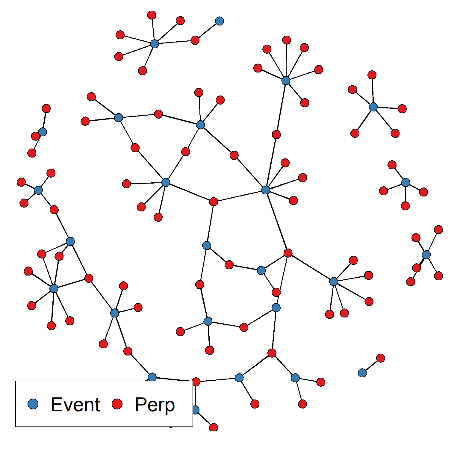
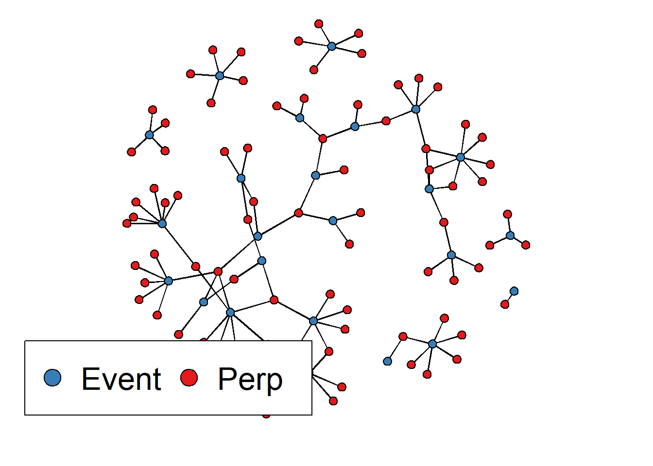
The BA-Bipartite kernel is the bipartite analogue of the BA kernel: the network has two disjoint node sets (say Part A and Part B), and edges may only occur across parts (A–B), never within a part.
At each event time \(t\), exactly one new node arrives, and it attaches to a subset of already-existing nodes in the opposite part using a normalized degree-based weighting (with optional aging / recency down-weighting).
Concretely:
Let \(V_A(t^-)\) and \(V_B(t^-)\) be the sets of existing nodes in Parts A and B just before time \(t\).
A single new node arrives in exactly one part (either A or B). Denote the new node by \(v_{\text{new}}\) and its part by \(P \in \{A,B\}\).
The candidate attachment targets are the old nodes in the other part: \[
V_{\text{opp}}(t^-) =
\begin{cases}
V_B(t^-) & \text{if } v_{\text{new}} \in A,\\
V_A(t^-) & \text{if } v_{\text{new}} \in B.
\end{cases}
\]
For each candidate target \(u \in V_{\text{opp}}(t^-)\), the new node attaches to \(u\)independently with probability \[
p_u(t) \propto (d_u(t^-) + \delta)\,\exp\!\big(-\beta_{\text{edges}}\cdot \text{age}_u(t)\big),
\] where \(d_u(t^-)\) is the current (bipartite) degree of \(u\) right before time \(t\), and \(\text{age}_u(t) = t - t_u\) is time since \(u\) arrived (from the stored node time attribute).
These weights are normalised over \(V_{\text{opp}}(t^-)\) to form Bernoulli probabilities, and the probability of observing a specific attachment set is a product of Bernoulli terms over the opposite-part node set: \[
\Pr(\text{attachments at } t) = \prod_{u \in V_{\text{opp}}(t^-)} p_u(t)^{I_u}\,(1-p_u(t))^{1-I_u},
\] where \(I_u=1\) if an edge between \(v_{\text{new}}\) and \(u\) is present at time \(t\), and \(I_u=0\) otherwise.
Intuitively:
Nodes in the opposite part with higher degree are more likely to receive a new tie (preferential attachment).
If \(\beta_{\text{edges}} > 0\), older nodes are down-weighted (recency/aging).
\(\delta\) is a small smoothing constant so degree-zero nodes remain eligible.
Data Expectations
To use the BA-Bipartite kernel, your observed events must represent a bipartite growth process where:
Each node belongs to exactly one of two parts (A or B).
Each event introduces exactly one new node (in either part).
Any edges observed at that event must connect the new node to already-existing nodes in the opposite part.
In particular, the BA-Bipartite kernel assumes:
No within-part edges (no A–A or B–B edges).
No old–old edges (edges cannot form between two already-existing nodes).
No new–new edges (the new node cannot connect to another node that arrives at the same event).
Within an event, you should not repeat the same attachment (no duplicate new–old pair).
Edge cases:
If the opposite part has no existing nodes yet (e.g. \(V_{\text{opp}}(t^-)=\emptyset\)), then the event must have no edges.
If your data contains edges between two already-existing nodes (e.g. repeated interactions/transactions), or edges within the same part, then this BA-Bipartite mark model is not an appropriate fit without extending the mark space / PMF.