set.seed(1)

time <- 50
params_ba_true <- list(
  mu = 0.5,
  K = 0.5,
  beta = 0.5,
  beta_edges = 2
)

sim <- sim_hawkesNet(
  params = params_ba_true,
  T_end = time,
  mark_type = "ba"
)
[1] "Simulation took 2.13 seconds"The BA kernel is a new-node attachment model: at each event time, exactly one new node arrives, and it connects to a subset of the already-existing nodes.
In the current hawkesNet implementation, the set of attachments is modelled as follows:
Intuitively:
Under this mark model, the probability of observing a particular set of attached old nodes is a product of Bernoulli terms over the old node set: \[ \Pr(\text{attachments at } t) = \prod_{u \in V(t^-)} p_u(t)^{I_u}\,(1-p_u(t))^{1-I_u}, \] where \(I_u = 1\) if the new node attached to \(u\), and \(I_u=0\) otherwise.
To use the BA kernel, your observed events must match the “new node arrives + connects to existing nodes” pattern:
Edge cases:
Simulate BA data:
set.seed(1)
time <- 50
params_ba_true <- list(
mu = 0.5,
K = 0.5,
beta = 0.5,
beta_edges = 2
)
sim <- sim_hawkesNet(
params = params_ba_true,
T_end = time,
mark_type = "ba"
)[1] "Simulation took 2.13 seconds"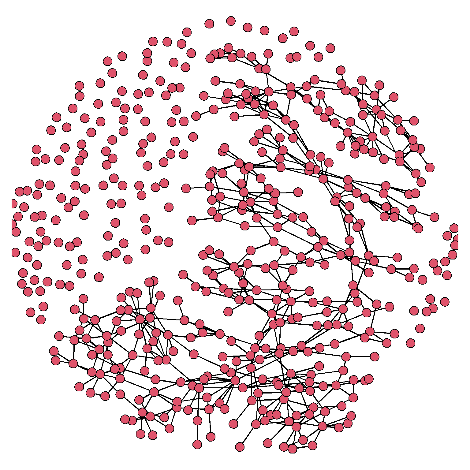
Fit BA data.
params_ba_init <- list(
  mu = 1,
  K = 1,
  beta = 1,
  beta_edges = 1
)

fit <- fit_hawkesNet(
      ev = sim$ev,
      params_init = params_ba_init,
      mark_type = "ba"
    )
[1] "Fitting took 5.55 seconds"Parameter values on the fitted scale:
unlist(fit$par) mu K beta beta_edges
1.4169583 0.4623329 0.5102294 2.0408620 Not too bad.
And, we can also grab parameter values on the transformed scale:
# Yes I know this is a jank way to structure it right now, will fix
fit$fit$par
mu K beta beta_edges
0.3485126 -0.7714700 -0.6728948 0.7133722