Quick summary
Accidentally messed up so the number of replicates for the last two sims are off.
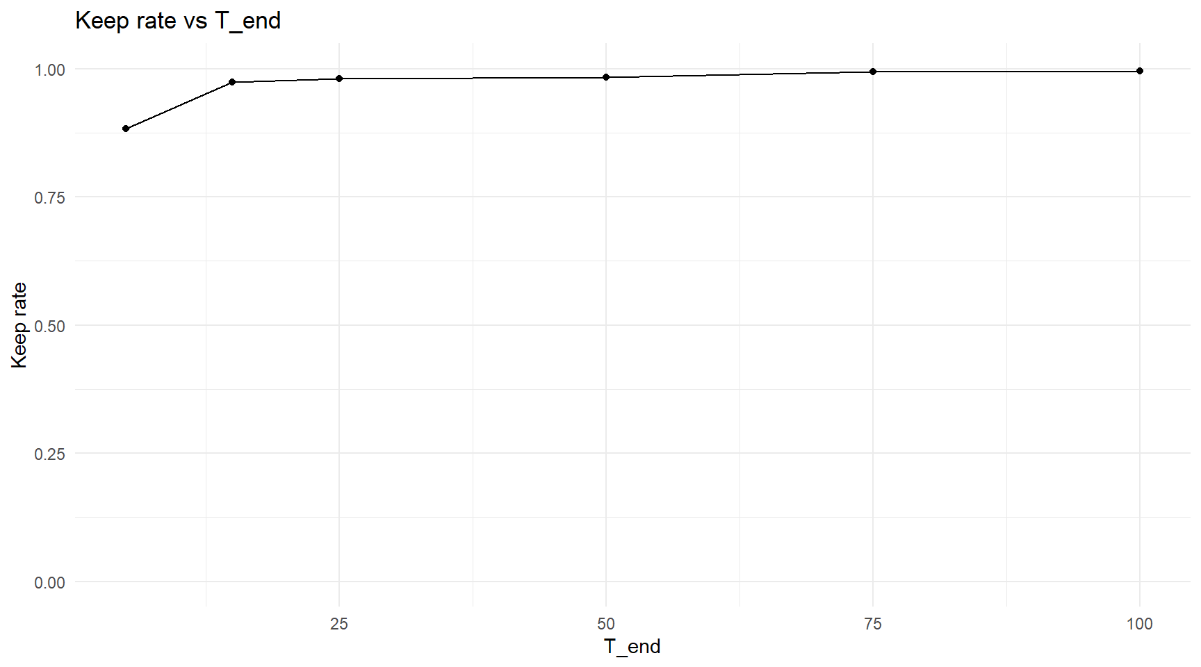
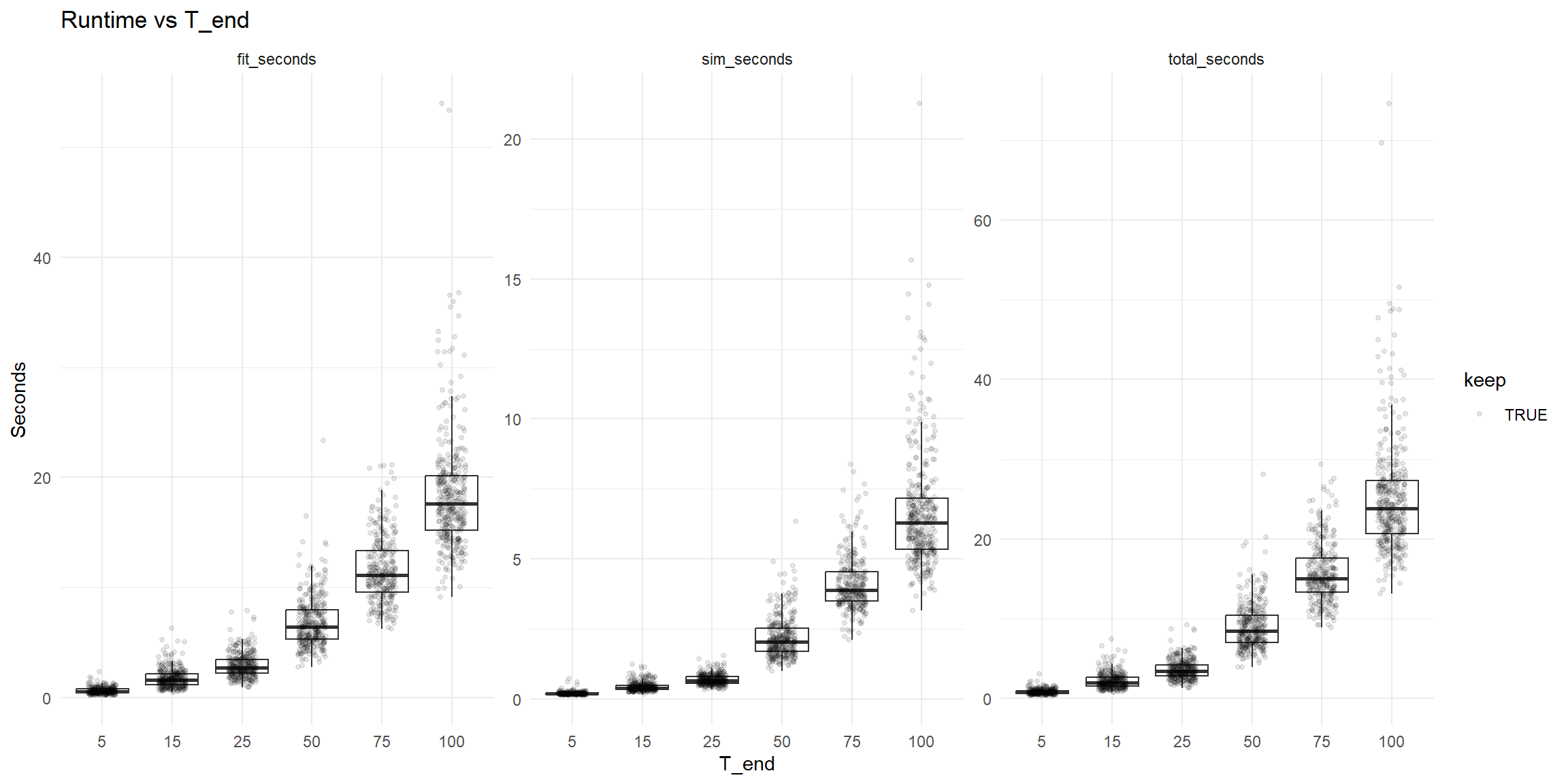
# A tibble: 6 × 7
  T_end     n keep_rate n_events_mean n_events_sd sim_s_mean fit_s_mean
  <dbl> <int>     <dbl>         <dbl>       <dbl>      <dbl>      <dbl>
1     5   350     0.883          20.4        7.43      0.208      0.636
2    15   350     0.974          69.0       16.0       0.445      1.78
3    25   350     0.98          118.        22.1       0.702      2.96
4    50   350     0.983         244.        30.1       2.20       6.94
5    75   310     0.994         368.        37.7       4.12      11.6
6   100   390     0.995         491.        43.1       6.66      18.5
Cap-Exceeded Replicates
Same as BA, filtering out explosive sims.
df %>%
  summarise(
    n_total = n(),
    n_keep  = sum(keep, na.rm = TRUE),
    n_dropped_caps = sum(drop_reason == "cap_exceeded", na.rm = TRUE)
  )
# A tibble: 1 × 3
  n_total n_keep n_dropped_caps
    <int>  <int>          <int>
1    2100   2033             67
df_non_filtered <- df


df <- df %>% filter(keep)
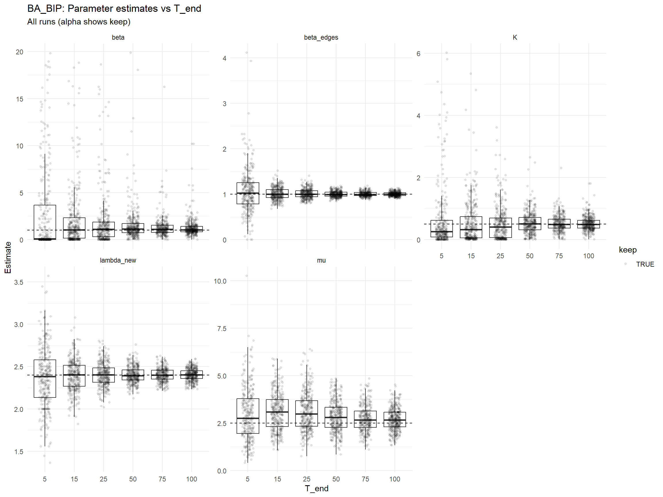
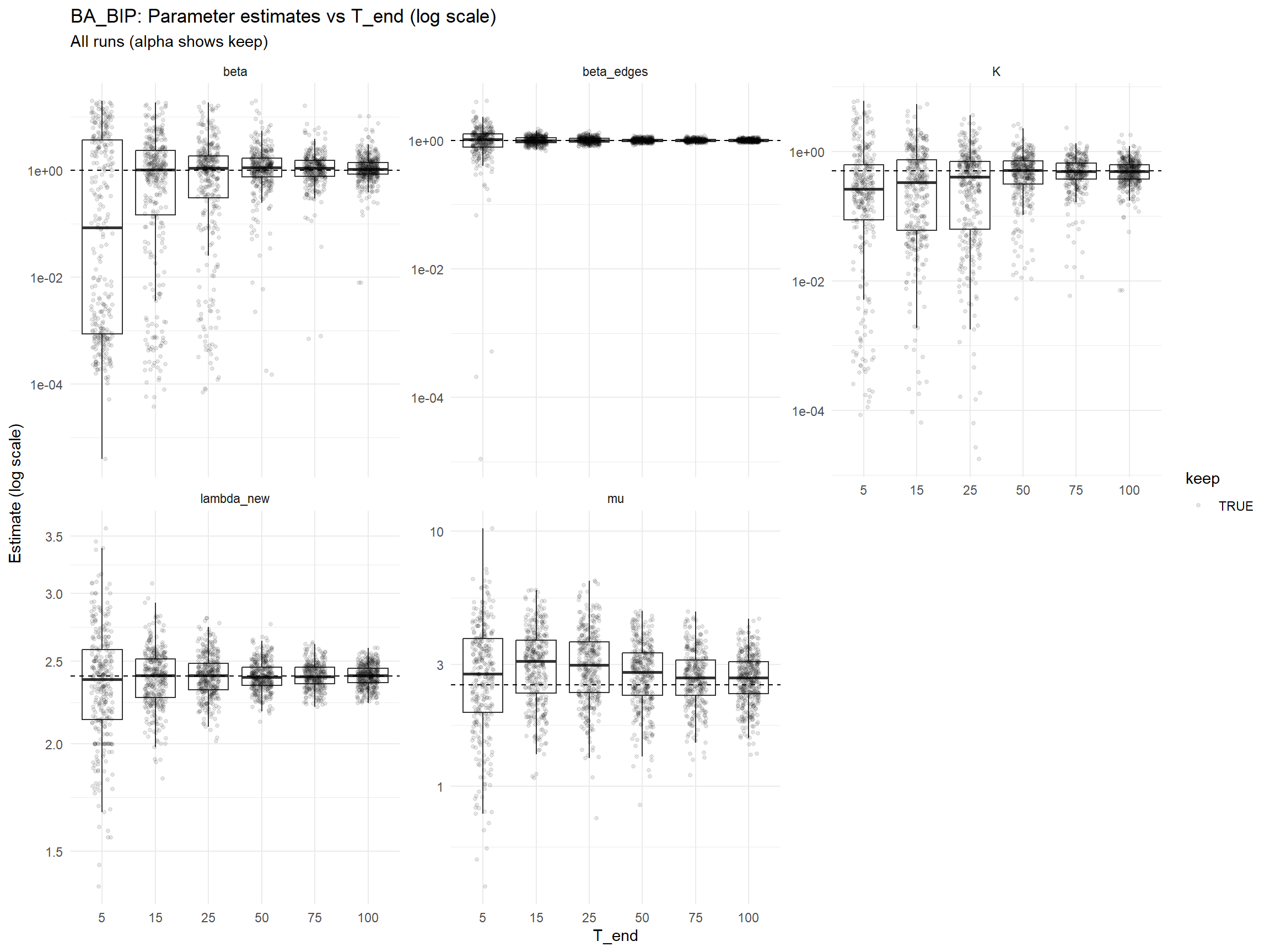
Parameter estimates vs T_end
Dashed line = true value.
plot_estimates_vs_T_ba_bip(df, log_scale = FALSE)
plot_estimates_vs_T_ba_bip(df, log_scale = TRUE)
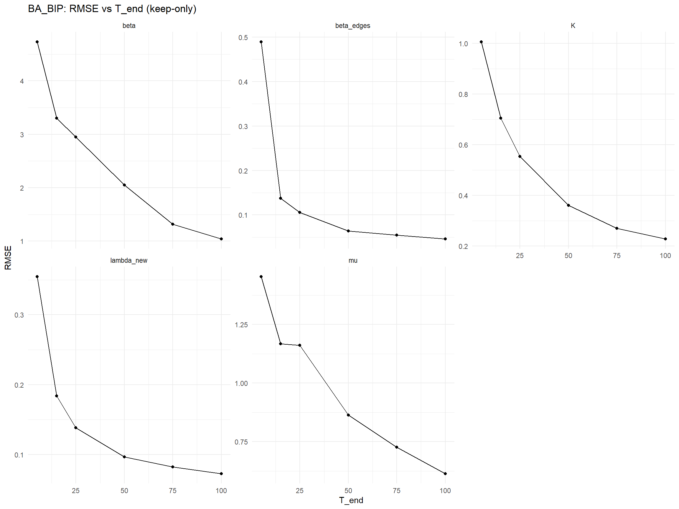
RMSE decay vs T_end
plot_rmse_vs_T_ba_bip(df)
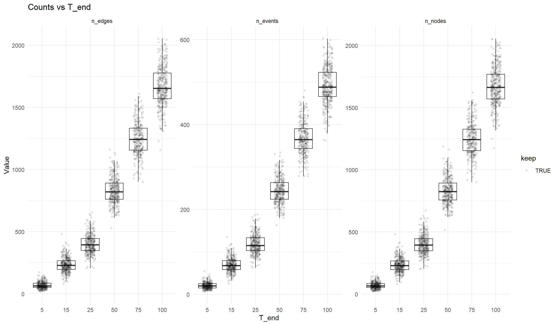
Keep rate vs T_end
plot_keep_rate_vs_T(df_non_filtered)